IOAI Training: Learn AI by solving problems

The problem in brief

A hiker is lost in a simulated mountain range. Before his radio died he sent only two numbers: his altitude (from an altimeter) and the compass bearing of the path he was on. You must choose, for each such reading, the point where a rescue helicopter lands. You get 1334 simulated training scenarios with the true position $(x, y)$ in metres plus the two readings, and 1335 test readings without positions. Your program prints one landing point per test reading (on Kattis the predictions are simply printed by the submitted program).

How you are scored

For one reading, the error is the area of the circle the team must search, with radius the distance between landing point and hiker:

\text{Error} = \pi\big((\hat x - x)^2 + (\hat y - y)^2\big),

averaged over the test readings. With $\text{baseline} = 1.7\times10^9$ and $\text{best} = 1.0\times10^9$ ,

\text{Score} = \max\Big(0, \min\Big(100,\ 100\,\frac{\text{baseline} - \text{mean error}}{\text{baseline} - \text{best}}\Big)\Big).

The baseline is exactly what you get by always landing at the average training position: $\pi(\operatorname{Var}x + \operatorname{Var}y) \approx 1.69\times10^9$ . The target, $10^9$ , means cutting the mean squared distance by 41 %. The test positions are private, so we evaluate by 5-fold cross-validation on the training set (repeated with two random splits).

The metric is a mean squared distance. That fact decides the whole approach: for squared error, the best single answer given the evidence is the conditional mean $\mathbb{E}[(x,y)\mid \text{readings}]$ , not the most likely point.

First look at the data

Plot the training positions and the structure jumps out.

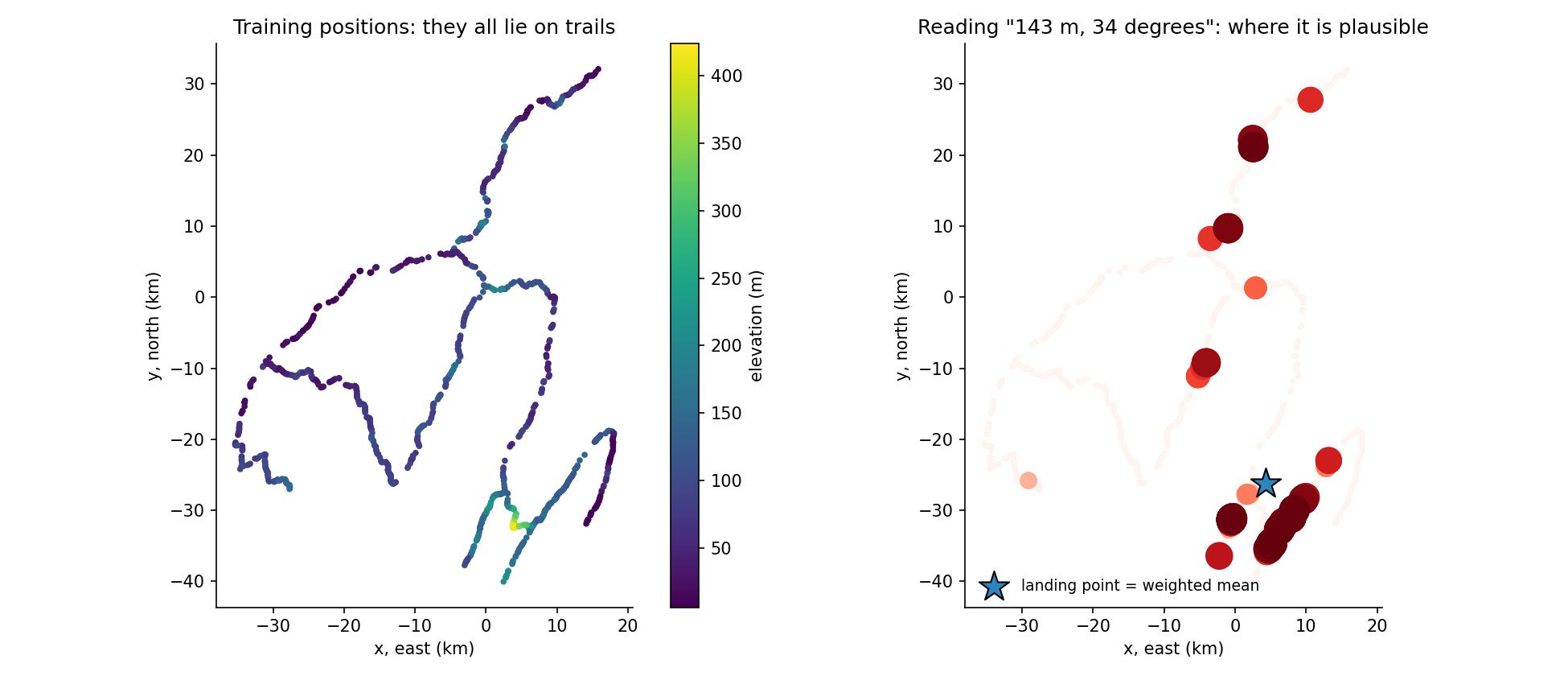
Left: the 1334 training positions coloured by elevation; they draw thin curves, a network of trails, with elevation varying smoothly along each trail. Right: for the test reading 143 m and 34 degrees, the trail points coloured by how plausible they are; plausible places form several separate clusters, and the weighted mean, marked by a star, lies between them.

The hiker is always on a trail. Positions are not spread over the map but lie on a few long curves. Neighbouring training points are typically 70 m apart.
Elevation varies smoothly along a trail: two neighbouring points differ by 2 m (median).
The compass gives the direction of the trail, up to a U-turn. Fitting a local line through each point's neighbours, the compass reading agrees with the trail's bearing modulo 180 degrees (median gap 12 degrees). Modulo 360 it does not: half of the neighbouring pairs point in opposite directions, because the hiker may walk either way. So the right feature for an angle $\theta$ is $(\cos 2\theta, \sin 2\theta)$ , not $\theta$ itself and not even $(\cos\theta, \sin\theta)$ .
A reading is ambiguous: an altitude of 143 m and a bearing of 34 degrees occur at several places on the network (right panel).

A first baseline

Landing at the mean position scores 0.7 (by construction). A k-nearest-neighbours regressor on the features $(e/20,\ \cos 2\theta,\ \sin 2\theta)$ , which looks for training readings similar to the test reading and averages their positions, already does much better: 74.7 with $k=20$ . A random forest on the same features gives the same 74.7. Note how bad small $k$ is (49.7 with $k=5$ ): averaging few neighbours throws away the hedging that squared error rewards.

The key idea

Think like a Bayesian. The unknown is the position $p$ on the trail network; the evidence is the reading $(e, \theta)$ . Bayes' rule gives

P(p \mid e,\theta) \propto P(p)\; \mathcal{N}(e;\ h(p),\ \sigma^2)\; \exp\big(\kappa\,(\cos 2(\theta - \alpha(p)) - 1)\big),

where $h(p)$ is the elevation and $\alpha(p)$ the trail bearing at $p$ , with Gaussian altimeter noise and an axial von Mises compass noise (the factor 2 makes $\theta$ and $\theta+180°$ equivalent). The training points are samples of the prior $P(p)$ , so the posterior mean is a weighted average of trail points:

\hat p = \frac{\sum_i w_i\, p_i}{\sum_i w_i},\qquad w_i = \exp\Big(-\frac{(e-e_i)^2}{2\sigma^2} + \kappa\big(\cos 2(\theta-\alpha_i) - 1\big)\Big).

This is kernel (Nadaraya-Watson) regression, but derived from a model of the measurement noise, which tells us which kernel to use. Why is the weighted mean optimal? For any landing point $c$ ,

\mathbb{E}\big[\lVert p - c\rVert^2 \mid \text{reading}\big] = \mathbb{E}\big[\lVert p - \hat p\rVert^2\big] + \lVert \hat p - c \rVert^2,

which is smallest at $c = \hat p$ . In the figure, the posterior has several clusters and the best landing point sits between them, possibly off any trail. Landing on the single most plausible spot would be a gamble that the squared metric punishes hard when it fails.

One more improvement comes from the trail structure: 1334 points leave gaps along the trails, and their compass readings are noisy. We densify the network: each point is joined to its 3 nearest neighbours closer than 800 m, the segment is sampled every 25 m with linearly interpolated elevation, and each sample receives the segment's bearing, which is less noisy than a single compass reading. The posterior is then computed on these dense samples.

The full solution

Read train.csv; convert directions to radians.
Densify the trails (about 25 m spacing) as described above.
For each test reading, compute the log-weights of all trail samples, subtract the maximum (numerical stability) and exponentiate:

logw = -(e - ed[None])**2 / (2 * S_ELEV**2) + KAPPA * (np.cos(2 * (th - ad[None])) - 1)
w = np.exp(logw - logw.max(1, keepdims=True))
pred = (w @ Pd) / w.sum(1, keepdims=True)          # posterior mean position

Choose $\sigma$ and $\kappa$ by cross-validation; the grid $\sigma\in\{2,3,4,5\}$ m, $\kappa\in\{2,3,4,5\}$ gives a flat optimum around $\sigma = 4$ m, $\kappa = 4$ (for $\kappa=4$ the doubled angle has a spread of about $1/\sqrt{\kappa} = 0.5$ rad, so about 15 degrees on the bearing itself, consistent with the 12-degree median gap measured above). The densification itself is retrained inside each fold, so the validation points never help build the trails they are scored on.
Print x y for each test row.

Results

5-fold cross-validation on the training set (the official test positions are private):

approach	mean error	score
land at the mean training position (baseline)	$1.69\times10^9$	0.7
kNN on $(e, \cos 2\theta, \sin 2\theta)$ , $k=5$	$1.35\times10^9$	49.7
kNN, $k=20$	$1.18\times10^9$	74.7
random forest, same features	$1.18\times10^9$	74.7
Bayesian kernel weights on training points ( $\sigma=8$ , $\kappa=5$ )	$1.17\times10^9$	75.5
same on the densified trail network (final)	$1.15\times10^9$	78.6 (79.5 and 77.7 on two splits)

We reach about 79 % of the way from the baseline to the reference solution. The remaining gap is mostly irreducible ambiguity: a reading often matches several distant stretches of trail, and no landing point can be close to all of them. Differences of one or two points between methods are within the noise of a 1334-point cross-validation (a few large errors dominate a squared metric).

What to remember

Plot the targets on a map before modelling. Seeing that every position lies on a trail turns a blind regression into a structured inference problem.
Under squared error, predict the conditional mean. When the posterior is multimodal, the optimal answer lies between the modes, not on the most likely one.
Kernel regression is Bayes in disguise: the kernel is the likelihood of the measurement noise, and the training points are samples of the prior.
Encode angles by what they mean. A direction that is ambiguous up to a U-turn lives on a circle of period 180 degrees: use $\cos 2\theta$ , $\sin 2\theta$ .
Exploit known structure to create data: interpolating along the trails gives a denser, cleaner prior than the raw samples.

"""SAIO "Lost in the Mountains": where should the helicopter land?

The training positions all lie on a network of trails, the altimeter reading
varies smoothly along a trail, and the compass reading is the trail's bearing
(walked in either direction, so it is only meaningful modulo 180 degrees).

Method = Bayesian posterior mean (the MSE-optimal point under squared distance):
  1. densify the trail network: join each training point to its 3 nearest
     neighbours (if closer than 800 m) and sample points every 25 m along the
     segments, interpolating the elevation; the bearing of a sample is the
     segment's bearing;
  2. weight every trail sample by the likelihood of the reading:
        w = exp(-(e - e_i)^2 / (2 s^2)) * exp(kappa (cos 2(theta - theta_i) - 1))
     (Gaussian altimeter noise, axial von Mises compass noise);
  3. predict the weighted mean position.
s = 4 m and kappa = 4 were chosen by 5-fold cross-validation (2 seeds).

Run:  python solution.py data/train.csv data/test.csv > answer.txt
      python solution.py data/train.csv --cv       (cross-validation report)
"""
import sys
import numpy as np
import pandas as pd
from sklearn.model_selection import KFold
from sklearn.neighbors import NearestNeighbors

S_ELEV, KAPPA, K_NEIGH, R_MAX, STEP = 4.0, 4.0, 3, 800.0, 25.0


def densify(P, elev):
    """Sample points every STEP metres along short segments joining neighbours."""
    dist, idx = NearestNeighbors(n_neighbors=K_NEIGH + 1).fit(P).kneighbors(P)
    pts, el, ang, seen = [], [], [], set()
    for i in range(len(P)):
        for j, dd in zip(idx[i, 1:], dist[i, 1:]):
            if dd > R_MAX or (j, i) in seen:
                continue
            seen.add((i, j))
            n = max(2, int(dd / STEP))
            t = np.linspace(0, 1, n, endpoint=False)[:, None]
            v = P[j] - P[i]
            pts.append(P[i] + v * t)
            el.append(elev[i] + (elev[j] - elev[i]) * t[:, 0])
            ang.append(np.full(n, np.arctan2(v[0], v[1])))   # compass bearing (0 = north)
    return np.vstack(pts), np.concatenate(el), np.concatenate(ang)


def predict(P, elev, e_q, th_q):
    Pd, ed, ad = densify(P, elev)
    out = np.zeros((len(e_q), 2))
    for s in range(0, len(e_q), 200):                   # chunks keep memory small
        e, th = e_q[s:s+200, None], th_q[s:s+200, None]
        logw = -(e - ed[None]) ** 2 / (2 * S_ELEV ** 2) + KAPPA * (np.cos(2 * (th - ad[None])) - 1)
        w = np.exp(logw - logw.max(1, keepdims=True))   # stable softmax
        out[s:s+200] = (w @ Pd) / w.sum(1, keepdims=True)
    return out


def error(pred, true):
    return np.pi * ((pred - true) ** 2).sum(1).mean()


def score(E):
    return max(0.0, min(100.0, (1.7e9 - E) / (1.7e9 - 1.0e9) * 100))


if __name__ == "__main__":
    tr = pd.read_csv(sys.argv[1])
    P = tr[["x", "y"]].values
    e = tr.elevation.values.astype(float)
    th = np.radians(tr.direction.values)
    if sys.argv[2] == "--cv":
        for seed in (0, 1):
            pred = np.zeros_like(P)
            for a, b in KFold(5, shuffle=True, random_state=seed).split(P):
                pred[b] = predict(P[a], e[a], e[b], th[b])
            base = np.tile(P.mean(0), (len(P), 1))
            print(f"seed {seed}: mean-position error {error(base, P):.3e}, "
                  f"ours {error(pred, P):.3e} -> score {score(error(pred, P)):.1f}")
    else:
        te = pd.read_csv(sys.argv[2])
        pred = predict(P, e, te.elevation.values.astype(float), np.radians(te.direction.values))
        print("\n".join(f"{x:.2f} {y:.2f}" for x, y in pred))