IOAI Training: Learn AI by solving problems

The problem in brief

You run a bank and receive one day of card purchases: for each of $N$ customers (900 to 3000) you know their age, gender, the shop, the product type, the GPS position of the purchase, the amount spent and the hour. A small share of these customers (2 to 3 % in the examples) are fraudsters, and you must output a 0/1 flag for every purchase. There is no training set: the hidden test cases are new days "with the same characteristics", so the program must discover by itself, on each input, what normal behaviour looks like. This is unsupervised anomaly detection. The task comes from the Swedish AI Olympiad qualifier 2025 (problem by Rasmus Hulthe), judged on Kattis with a 2-second CPU limit; NumPy is available, scikit-learn is not.

Two local test cases are attached with their labels (3196 and 2335 rows). We use them only to understand the data and to evaluate; the Kattis test cases are hidden.

How you are scored

On each test case, with $TP$ the percentage of fraudsters you catch and $FP$ the percentage of honest customers you wrongly flag:

\text{Score} = \max\big(0,\ TP - 5\cdot FP\big),

averaged over test cases. A false alarm costs five times as much as a missed fraudster (in percentage points), and since honest customers are about 35 times more numerous, flagging one honest customer out of 3000 already costs 0.17 points. The rule pushes you towards a very conservative threshold.

What to aim for. There is no official threshold. The problem's public statistics page on Kattis shows one full solve (100 points) and then 59.1, 58.4 and 54.4 as the next best scores, so anything above 60 beats almost every contestant.

First look at the data

A first surprise: the two local test cases do not live in the same world. Case 1 is centred near latitude 41.8, case 2 near 39.8; ages range over 18 to 70 in one and 14 to 102 in the other; the typical amounts and hours also move. A model trained on one day and applied to another would fail. Whatever we do has to be re-fitted on each input.

Then look at each column on its own, honest versus fraud:

Gender, product type and shop: fraud rates are flat across categories (between 2 and 4 % everywhere), pure noise.
Age, latitude, longitude: the two distributions overlap almost perfectly.
Amount and hour: honest purchases are bimodal (two habits, for example "around 600 in the evening" and "around 1500 in the morning"), and fraudsters are not more extreme than honest customers on either axis taken alone.

The picture changes completely when you plot hour against amount together:

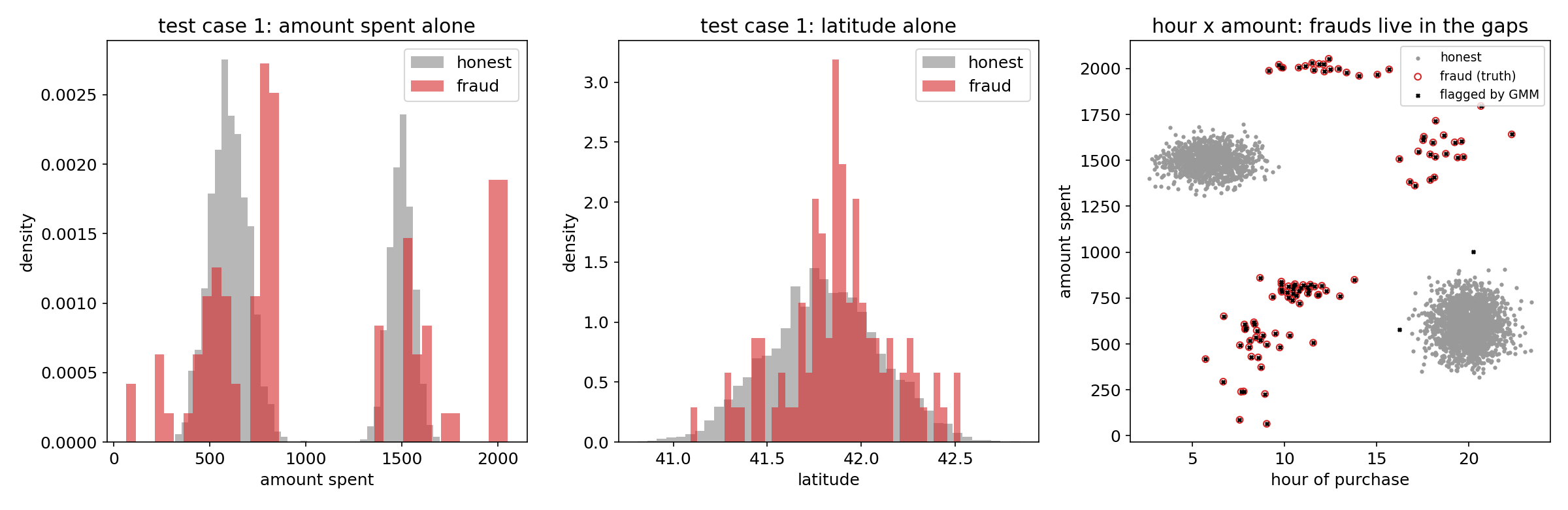
Amount and latitude alone do not separate frauds; hour x amount does

Honest customers form two dense, round clouds. Fraudsters form small loose clusters in the empty space between them. A fraudster buying for 800 at 10 am is not unusual in amount (honest people spend 800) nor in hour (honest people shop at 10), only the combination never occurs among honest customers.

A first baseline

approach	case 1	case 2
flag nobody (provided baseline)	0	0
flag $\lvert z\rvert > 3$ on amount, or on hour	0	0
Isolation Forest on all 5 numeric columns, contamination 3 %	21.8	34.1
Isolation Forest on (hour, amount) only, contamination 3 %	96.4	94.2

Single-feature z-scores catch nothing, as the histograms predicted: frauds are not in the tails. An Isolation Forest (via scikit-learn, so not submittable, but a useful reference) is poor with all columns, because age and GPS are pure noise and dilute the isolation paths, and very good once restricted to the two informative columns. Choosing the right space matters more than the anomaly detector. The remaining weakness is the fixed "3 % contamination": it forces a fixed number of flags whatever the data says.

The key idea

Model normal behaviour explicitly as a mixture of Gaussians in the (hour, amount) plane, then flag what no normal component explains.

A Gaussian mixture with $k$ components has density

p(\mathbf{x}) = \sum_{j=1}^{k} w_j\,\mathcal{N}(\mathbf{x}\mid \boldsymbol\mu_j,\Sigma_j),

fitted by the EM algorithm. With several components, the fraud clusters themselves get small components; the honest habits get large and dense ones. We call a component "normal" if its weight is at least 5 % and its peak density $w_j/\sqrt{\det\Sigma_j}$ is at least a tenth of the densest one (this second test matters when EM lumps several scattered fraud clusters into one wide component).

For a point $\mathbf{x}$ , the squared Mahalanobis distance to a component,

d_j^2(\mathbf{x}) = (\mathbf{x}-\boldsymbol\mu_j)^\top \Sigma_j^{-1} (\mathbf{x}-\boldsymbol\mu_j),

follows a $\chi^2$ distribution with 2 degrees of freedom if $\mathbf{x}$ really comes from that component. That gives a threshold with a meaning: flagging $\min_j d_j^2 > 13.82$ (the 99.9 % quantile of $\chi^2_2$ ) wrongly flags about 0.1 % of honest customers, which costs about $5 \times 0.1 = 0.5$ points. The 5x penalty is exactly why we choose a tail probability this small, rather than a "contamination" rate guessed in advance. The number of flags now adapts to each input.

The full solution

Read only the amount and hour lines (the other six are noise), and standardise both axes (median, standard deviation) so that EM sees round clusters.
Fit mixtures with $k = 1,\dots,5$ components, two k-means++ restarts each, 80 EM iterations, and keep the one with the lowest BIC, $-2\log L + p\log N$ , which balances fit against the number of parameters $p$ .
Mark the large and dense components as normal behaviour.
Flag every customer whose squared Mahalanobis distance to the nearest normal component exceeds 13.82.

The EM step is a few lines of NumPy:

L = np.stack([log_gauss(X, mu[j], S[j]) + np.log(w[j]) for j in range(k)], 1)
R = np.exp(L - L.max(1, keepdims=True)); R /= R.sum(1, keepdims=True)  # responsibilities
Nk = R.sum(0); w = Nk / n; mu = (R.T @ X) / Nk[:, None]                # M-step

The whole program runs in 0.5 s on 3200 rows, well inside the 2 s limit.

Robustness check. Two local cases are a tiny sample, so we also generated 40 synthetic days of our own (2 or 3 honest clusters with random weights, 2 to 4 % fraud in small clusters placed anywhere outside the honest clouds). The method averages 97.7, with a median of 99.5. Its failure mode is instructive: when a genuine honest habit holds only about 9 % of customers, it can be mistaken for fraud, and flagging a whole honest cluster costs about 45 points. Synthetic data is our guess of "the same characteristics", not the official generator.

Results

Scores on the two labelled local test cases (the official Kattis tests are hidden).

approach	case 1	case 2
flag nobody	0	0
z-score $>3$ on one column	0	0
Isolation Forest, all numeric columns	21.8	34.1
Isolation Forest, (hour, amount)	96.4	94.2
GMM on (hour, amount, latitude, longitude), $\chi^2$ 99.9 %	99.7	97.9
GMM on (hour, amount), $\chi^2$ 99 %	95.0	95.0
GMM on (hour, amount), $\chi^2$ 99.99 %	100.0	97.9
GMM on (hour, amount), $\chi^2$ 99.9 % (final)	99.7	99.6

The final program catches every fraudster in both cases and raises 2 false alarms in each (0.06 % and 0.09 % of honest customers). Average: 99.6 on the local cases.

What to remember

Anomalies are often unusual combinations, not extreme values: always look at pairs of features, not only histograms.
Throwing in noise features hurts unsupervised detectors (Isolation Forest dropped from 96 to 22); feature selection by looking at the data is half the work.
When the test distribution shifts from case to case, fit the model on each input instead of training once.
A Gaussian model turns a threshold into a probability: $d^2 \sim \chi^2_d$ lets you pick the false-alarm rate that the scoring rule asks for (here very low, because of the 5x penalty).
BIC chooses the number of mixture components without labels.

"""SAIO Fraudster: unsupervised fraud flagging with a Gaussian mixture on (hour, amount).

Kattis submission (Python 3 with NumPy): reads the 9-line input from stdin, prints 0/1 flags.
Local check:  python3 solution.py --eval work/local_testcase_1.csv work/local_testcase_2.csv
"""
import sys
import numpy as np

CHI2_2DOF_999 = 13.8155   # 99.9 % quantile of chi-square with 2 degrees of freedom
MIN_WEIGHT = 0.05         # a mixture component with >= 5 % of customers is "normal behaviour"


def log_gauss(X, mu, S):
    D = X - mu
    Si = np.linalg.inv(S)
    return (-0.5 * np.einsum('ij,jk,ik->i', D, Si, D)
            - 0.5 * np.log(np.linalg.det(S)) - np.log(2 * np.pi))


def fit_gmm(X, k, rng, iters=80):
    """Plain EM for a k-component Gaussian mixture with full covariances, k-means++ start."""
    n, d = X.shape
    centres = [X[rng.integers(n)]]
    for _ in range(k - 1):
        d2 = np.min(((X[:, None] - np.array(centres)[None]) ** 2).sum(-1), 1)
        centres.append(X[rng.choice(n, p=d2 / d2.sum())])
    mu = np.array(centres)
    S = np.array([np.cov(X.T) * 0.1 + 1e-3 * np.eye(d)] * k)
    w = np.ones(k) / k
    for _ in range(iters):
        L = np.stack([log_gauss(X, mu[j], S[j]) + np.log(w[j]) for j in range(k)], 1)
        m = L.max(1, keepdims=True)
        R = np.exp(L - m)
        tot = R.sum(1, keepdims=True)
        loglik = (m[:, 0] + np.log(tot[:, 0])).sum()
        R /= tot
        Nk = R.sum(0) + 1e-9                      # E-step done, M-step below
        w = Nk / n
        mu = (R.T @ X) / Nk[:, None]
        for j in range(k):
            D = X - mu[j]
            S[j] = (R[:, j, None] * D).T @ D / Nk[j] + 1e-4 * np.eye(d)
    return w, mu, S, loglik


def flag_fraud(hour, amount, kmax=5, restarts=2):
    X = np.column_stack([hour, amount]).astype(float)
    X = (X - np.median(X, 0)) / X.std(0)          # put both axes on the same scale
    n, d = X.shape
    rng = np.random.default_rng(0)
    best = None
    for k in range(1, kmax + 1):                  # choose the number of components by BIC
        for _ in range(restarts):
            w, mu, S, ll = fit_gmm(X, k, rng)
            n_params = k * (d + d * (d + 1) / 2) + k - 1
            bic = -2 * ll + n_params * np.log(n)
            if best is None or bic < best[0]:
                best = (bic, w, mu, S)
    _, w, mu, S = best
    # a "normal habit" is a component that is both large and dense: fraud clusters are tiny,
    # and when EM lumps several of them together the result is large but very spread out
    peak = w / np.sqrt(np.linalg.det(S))
    normal = (w >= MIN_WEIGHT) & (peak >= 0.1 * peak.max())
    # squared Mahalanobis distance to the closest LARGE component (= a normal habit)
    d2 = np.min(np.stack([np.einsum('ij,jk,ik->i', X - mu[j], np.linalg.inv(S[j]), X - mu[j])
                          for j in range(len(w)) if normal[j]], 1), 1)
    return (d2 > CHI2_2DOF_999).astype(int)


def main_kattis():
    lines = sys.stdin.read().split('\n')
    n = int(lines[0])
    amount = np.array(lines[4].split(), dtype=float)
    hour = np.array(lines[7].split(), dtype=float)
    print(' '.join(map(str, flag_fraud(hour, amount)[:n])))


def score(y, p):
    tp = 100 * ((p == 1) & (y == 1)).sum() / (y == 1).sum()
    fp = 100 * ((p == 1) & (y == 0)).sum() / (y == 0).sum()
    return max(0.0, tp - 5 * fp), tp, fp


if __name__ == '__main__':
    if len(sys.argv) > 2 and sys.argv[1] == '--eval':
        import pandas as pd
        for f in sys.argv[2:]:
            df = pd.read_csv(f)
            p = flag_fraud(df.Time.values, df.Amount.values)
            s, tp, fp = score(df.Label.values, p)
            print(f'{f}: score {s:.2f}  (TP {tp:.1f} %, FP {fp:.2f} %)')
    else:
        main_kattis()