Colorize

The problem in brief

You receive 2,871 photos of 128x128 pixels (from the Yahoo Flickr Creative Commons collection) together with their grayscale versions, and 1,547 grayscale test photos whose colours were lost. You must predict the colour of every 131st pixel of the test images (counting pixels across all images in a fixed order) and print the R, G, B values as integers; the printed list is the submission. The hidden original colours are scored by mean squared error. The task comes from the final of the Swedish AI Olympiad 2026 (saio.kattis.com/problems/colorize); the test colours are private, so we score on 15 % of the training pairs held out from training (446 images).

How you are scored

With $g_i$ the predicted and $t_i$ the true value over all evaluated R, G and B entries,

$$\text{MSE} = \frac{1}{N}\sum_{i=1}^{N}(g_i - t_i)^2 , \qquad \text{Score} = 100\cdot\operatorname{clip}\left(\frac{666 - \text{MSE}}{99},\,0,\,1\right).$$

So an MSE of 666 or more earns nothing and 567 or less earns full marks. The organisers' baseline, which copies the gray value into all three channels, scores 696 on our validation images: below zero points. The target is to cut the error of "no colour at all" by about a fifth.

First look at the data

• The gray image is exactly the luma. On every training pair, the gray value equals $Y = 0.299R + 0.587G + 0.114B$ of the colour image (mean absolute difference 0.2 gray levels, JPEG noise). That is the standard conversion, and it means the brightness of each pixel is known: only its colour (hue and saturation) must be guessed.
• Colour has a strong average. The mean colour offset from gray over all training pixels is $(+8.1, -1.8, -11.8)$ for (R, G, B): photos are on average warm, slightly yellow-orange. Adding this constant shift lowers the MSE from 696 to 616.5 (50 points). Making the shift depend on the gray level (the mean offset of all training pixels with that gray value, a 256-entry lookup table) gives 599 (67 points): dark pixels tend to be brownish, bright ones bluish-white like the sky.
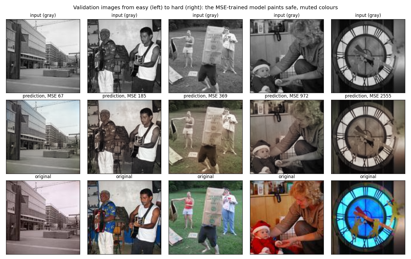
• The error is dominated by colourful images. Per-image MSE of our final model ranges from below 70 (gray buildings) to over 2,500 (a cyan illuminated clock). A few vivid, unpredictable images weigh as much as dozens of easy ones.

The key idea

Two observations shape the solution.

1. Predict only what is unknown, and keep the luma exact. Write each colour as the gray value plus two chroma components, $C_r = R - Y$ and $C_b = B - Y$. Given $Y$ (the input) and the two chroma values, the green channel follows from the luma equation:

$$R = Y + C_r, \qquad B = Y + C_b, \qquad G = Y - \frac{0.299\,C_r + 0.114\,C_b}{0.587}.$$

The network outputs two numbers per pixel instead of three, and every prediction has exactly the right brightness, so no capacity is wasted relearning it.

2. Under MSE, the best guess is the conditional mean, which is a muted colour. For a pixel whose colour is uncertain (a sweater could be red, blue or green), the prediction minimising the expected squared error is the average of the possible colours, which is close to gray-brown. A model trained with the MSE loss learns exactly that: it paints confident colours where the content is unambiguous (grass, sky, skin, wood) and stays cautious elsewhere. The colourisations look dull, but that is what the metric rewards. A model that produces vivid, "realistic" colours (for instance with an adversarial loss) would be punished hard whenever it picks the wrong hue: predicting red for a blue sweater costs far more than predicting gray. Choose the loss that is the metric.

Context is what makes the conditional mean sharp: knowing that a region is grass, sky or a face requires recognising objects, so we use a convolutional network with an ImageNet-pretrained encoder.

A first baseline and the model

The lookup table by gray level (MSE 599) is the natural non-neural baseline. The model is a U-Net:

• Encoder: ResNet-18 with ImageNet weights, applied to the gray image copied into three channels (normalised like ImageNet), giving feature maps at 1/2, 1/4, 1/8, 1/16 and 1/32 of the resolution.
• Decoder: five upsampling stages, each concatenating the encoder features of the same resolution (skip connections) and the gray image itself at full resolution, then two 3x3 convolutions; a final 1x1 convolution outputs $C_r$ and $C_b$.
• Training: loss = MSE between the reconstructed RGB image and the original (the metric itself), AdamW with a one-cycle schedule (peak learning rate $3\times10^{-4}$ for the pretrained encoder, $10^{-3}$ for the decoder), batch 32, random horizontal flips; at test time the prediction is averaged with that of the mirrored image. One epoch over the 2,425 training images takes about 10 s on an Apple laptop GPU.

The skip connections matter: colour must be placed precisely at object boundaries, and the deep features alone (4x4 pixels at the bottleneck) know what the objects are but not exactly where their edges lie.

The full solution

1. Read the training pairs and the test images in sorted filename order.
2. Train the U-Net for 15 epochs on 85 % of the pairs and check the validation MSE; then retrain the same configuration on all 2,871 pairs.
3. Predict the test images (with mirror averaging), clip to $[0, 255]$ and round to integers.
4. Write out.py, which prints the R G B values of every 131st pixel in the official order (global counter over images, $x$ in the outer loop, $y$ in the inner loop), exactly like the organisers' baseline: 193,481 pixels, 580,443 integers.

cr, cb = chroma[:, 0], chroma[:, 1]                      # network output
rgb = torch.stack([g + cr, g - (0.299 * cr + 0.114 * cb) / 0.587, g + cb], 1)
loss = F.mse_loss(rgb, true_rgb)                          # the competition metric itself

Results

Validation MSE on 446 held-out training pairs, over all pixels (the official every-131st-pixel sample gives nearly the same value, for example 528.7 against 527.2 for the final model).

approach	validation MSE	score
copy gray into R, G, B (organisers' baseline)	695.9	0
constant colour shift	616.5	50.0
mean shift per gray level (lookup table)	598.9	67.8
U-Net with randomly initialised encoder, 30 epochs	567.9	99.1
U-Net with ImageNet ResNet-18 encoder, 30 epochs	533.1	100
U-Net with ImageNet ResNet-18 encoder, 15 epochs (final)	527.2	100

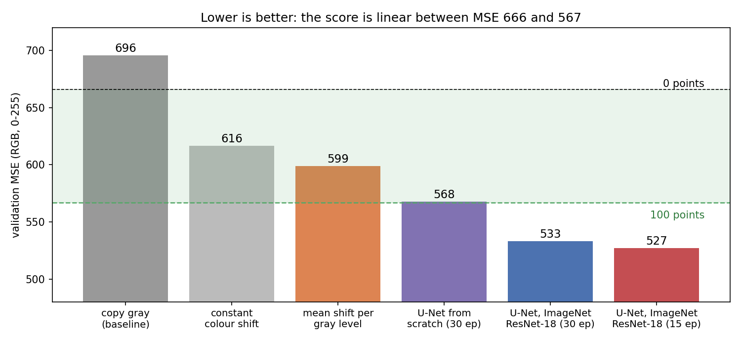
The pretrained encoder is worth 35 points of MSE over training from scratch: 2,871 images are too few to learn object recognition, but ImageNet features already know grass from sky. With 30 epochs the training MSE (about 200) falls far below the validation MSE: the model starts memorising the training images, which is why the shorter schedule generalises slightly better. With a margin of 40 below the full-marks threshold, the result should be robust to the difference between our validation images and the hidden test set.

What to remember

• Decompose the target into what is known and what is not. The gray input is the luma, so predict only the two chroma channels and reconstruct RGB exactly.
• Train on the metric. Under squared error the optimal prediction is the conditional mean, so muted colours are not a failure but the right answer to an MSE question; vivid generative colourisation would score worse.
• Climb the ladder of baselines. Constant shift, then a lookup table by gray level, then a network: each step tells you how much structure is left to exploit.
• Pretrained encoders transfer to dense prediction. A U-Net with an ImageNet backbone and skip connections combines "what is this object" with "where exactly is its edge".
• Reproduce the output format exactly. The global pixel counter across images and the $x$-before-$y$ loop order are easy to get wrong; reuse the organisers' loop.