IOAI Training: Learn AI by solving problems

The problem in brief

Camera traps in Russian nature reserves take photos whenever something moves, and zoologists have labelled 40,158 of them with one of 21 species: two bears, wild boar, four deer (Manchurian wapiti, sika deer, maral, Siberian roe deer), badger, sable, three small or large cats, tiger, snow leopard, argali, ibex, wolf, fox, raccoon dog, hare and marmot. You must label 16,342 test photos. Many photos are taken at night in infrared, are blurred, or show only part of an animal, and some species look very much alike. The data come from the organisers' public Yandex Disk folder. The test labels are private (they were scored on the contest platform), so everything below is measured on a held-out part of the training set.

How you are scored

The metric is macro F1: an F1 score is computed for each of the $K = 21$ classes, and the scores are averaged with equal weights:

F_1^{(k)} = \frac{2\,P_k R_k}{P_k + R_k}, \qquad \text{macro-}F_1 = \frac{1}{K}\sum_{k=1}^{K} F_1^{(k)} ,

where $P_k$ and $R_k$ are the precision and recall of class $k$ . The test set was split 40/60 into a public and a private leaderboard. The statement gives no threshold, and we found no public leaderboard, so there is no published target.

Macro averaging matters a lot here. Sika deer make up 41 % of the photos and sable only 0.3 % (136 images), but both count for $1/21$ of the score. A model that ignores the rare species can reach 97 % accuracy and still lose several points of macro F1.

First look at the data

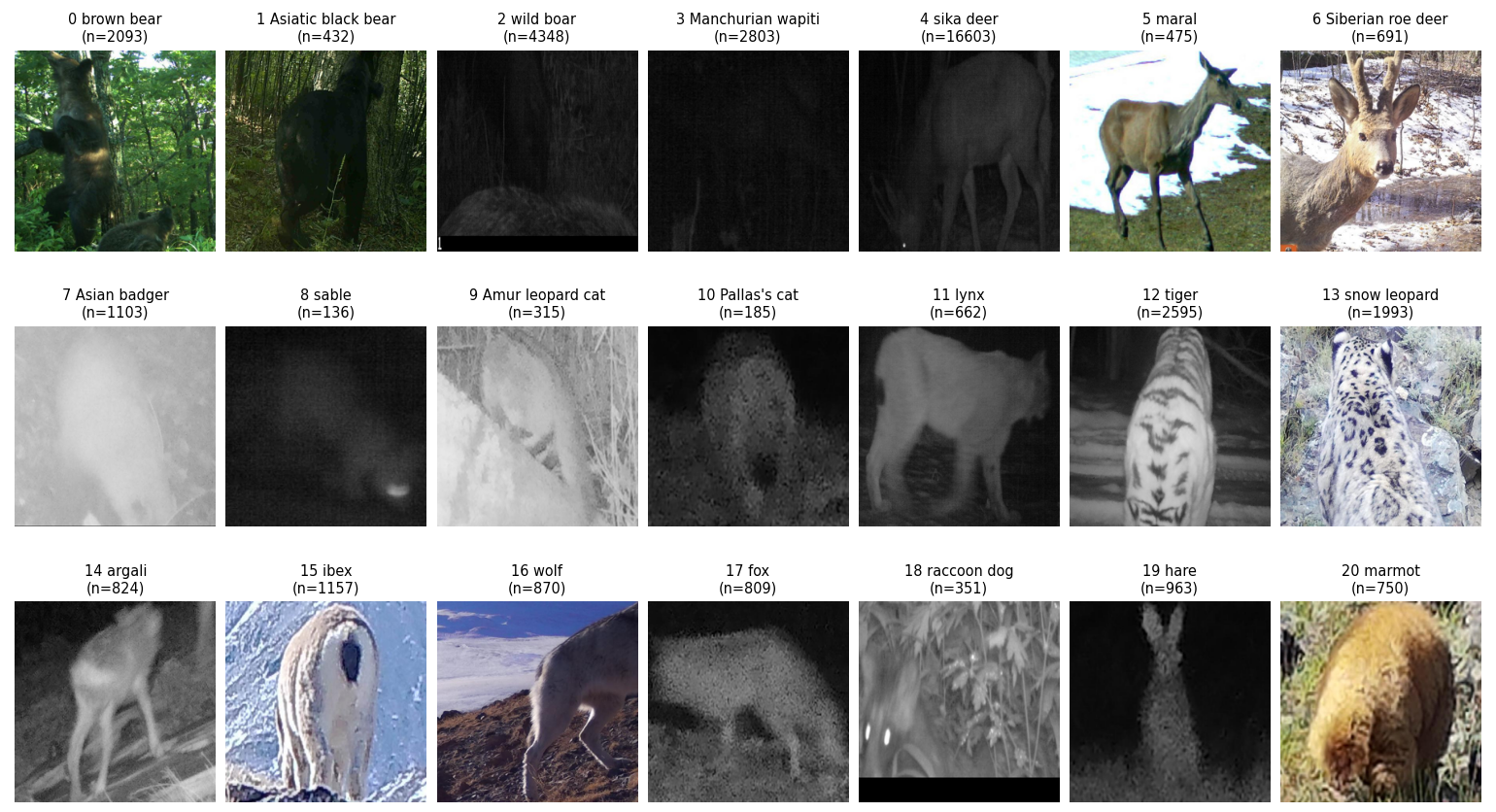
One random training photo per species, with the number of training images. Many are night infrared shots; the images are already crops around the animal, all 512x512.

The images are already cropped around the animal, all at 512x512 pixels. There is no detection step to do: this is a pure classification problem.
The classes are very unbalanced: from 16,603 sika deer down to 136 sable and 185 Pallas's cats.
Many photos come in bursts. A camera fires several frames in a row, so the training set contains groups of almost identical images. If two frames of the same burst land on both sides of a random train/validation split, the validation score is inflated. The file names are hashes and there is no metadata, so we rebuilt the bursts ourselves (see below).

A first baseline

Training a CNN from scratch on 40,000 images is slow on a laptop and wastes the most useful resource available: pretrained vision models. The statement explicitly allows public models and datasets, and the organisers' own baseline finetunes an ImageNet ResNet-18.

Our first baseline is even cheaper: we use DINOv2 ViT-S/14 (a self-supervised vision transformer) as a frozen feature extractor. Each image is resized to 224x224, the network gives a 384-dimensional CLS token and 256 patch tokens; we keep the CLS token concatenated with the mean of the patch tokens (768 numbers), averaged over the image and its mirror image. Then we train a linear softmax classifier on these vectors.

Linear head on ViT-S features: 0.864 macro F1 (92.7 % accuracy) on our grouped validation split.

Feature extraction takes about 8 minutes for the whole training set on an Apple laptop GPU, and the head trains in seconds, so every later idea is cheap to test.

The key idea

Two ideas carry the solution: a strong frozen representation with a small non-linear head, and an honest validation split.

Why frozen self-supervised features work. DINOv2 was trained on 142 million images to produce features in which similar-looking objects lie close together, without any labels. A camera-trap photo of a tiger, even in infrared, lands near other tigers. The classification problem then lives in a fixed 768- or 1536-dimensional space, where a small model trained on 32,000 examples is enough. Two improvements over the baseline matter:

A one-hidden-layer MLP instead of a linear head (1024 GELU units, dropout, label smoothing 0.1, AdamW with a one-cycle schedule, 40 epochs). Species are not linearly separable in the frozen space, especially at night; the MLP lifts the small model from 0.864 to 0.921.
A bigger encoder: DINOv2 ViT-B/14 (768-dimensional tokens, 1536 features) lifts the MLP to 0.937. It costs 25 minutes of extraction for the training set instead of 8.

Class weights for macro F1. The cross-entropy weights each class by $w_k = \sqrt{N / (K\,n_k)}$ , where $n_k$ is the number of training images of class $k$ . Full inverse-frequency weights ( $1/n_k$ ) would make one sable photo worth 120 sika deer and overfit the rare classes; the square root is a common compromise that pushes the decision boundaries towards the rare species without wrecking the frequent ones.

An honest validation split. To find the bursts, we normalise all feature vectors, compute all pairwise cosine similarities (in blocks of 2048 rows), link the pairs above 0.9, and take the connected components of that graph. About 34 % of the images fall into groups of two or more (the largest group, 250 to 390 images depending on the features, gathers very similar dark night frames). We then put 20 % of the groups, not of the images, into validation. On this data the effect turned out to be small (0.932 random split against 0.932 grouped for the ViT-S MLP), which tells us bursts are short and the photos varied enough; but it is the kind of check that must be done, because on other camera-trap data the gap can be large.

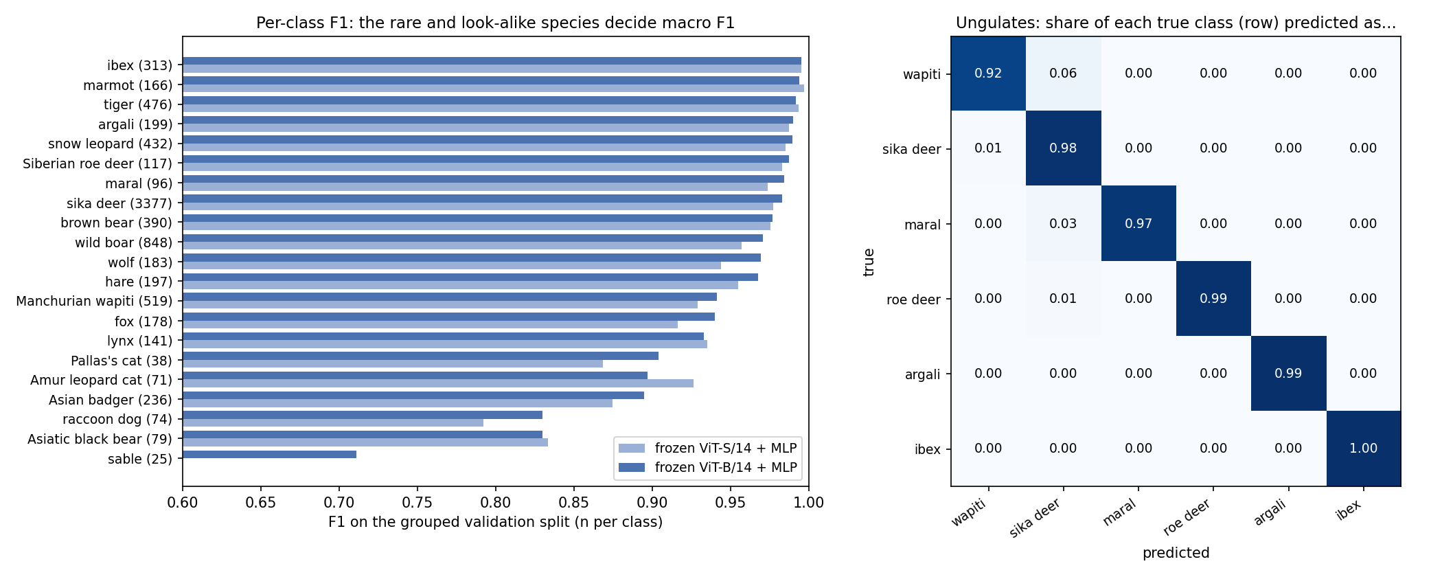
Left: per-class F1 on the grouped validation split, with the number of validation images per class. The small model's sable F1 (0.53) is off the left edge. Right: among the hoofed animals only wapiti and sika deer are really confused.

The per-class picture is instructive. The statement warns about the four deer, but the model separates them well: maral, roe deer, argali and ibex are all above 0.98, and only wapiti and sika deer get mixed (6 % of wapiti photos are called sika). The real weak spots are the rare night species: sable (25 validation images, F1 0.71), the Asiatic black bear (often confused with the brown bear in the dark), raccoon dog and badger. With 25 sable images, a single error moves that class's F1 by about 0.04, and macro F1 by 0.002: the validation estimate itself is noisy to about $\pm 0.01$ .

The full solution

Features. DINOv2 ViT-B/14 (timm, safetensors weights from Hugging Face), images resized to 224, position embeddings resampled from the 37x37 grid of the 518-pixel checkpoint to 16x16. Feature = [CLS, mean of patch tokens], averaged with the horizontally flipped image (test-time augmentation). Cached as float16 arrays.
Head. Standardise the features, then MLP (dropout 0.2, linear 1536 to 1024, GELU, dropout 0.3, linear to 21), square-root class weights, label smoothing 0.1, AdamW (learning rate $10^{-3}$ , weight decay $10^{-4}$ ), one-cycle schedule, 40 epochs of batches of 256. Three seeds, probabilities averaged.
Validation. 20 % of the near-duplicate groups held out, as described above.
Submission. Retrain the three heads on all 40,158 images and predict the test set.

tok = model.forward_features(x)                         # (B, 1 + 256, 768)
feat = torch.cat([tok[:, 0], tok[:, 1:].mean(1)], 1)    # CLS + mean patch token
# ... the same on torch.flip(x, dims=[3]), then average the two

Results

All scores are on a held-out 20 % of the training set (the official test labels are private), split by near-duplicate groups.

approach	macro F1	accuracy
ViT-S/14 frozen, linear head	0.864	0.927
ViT-S/14 frozen, MLP head (3 seeds)	0.921	0.963
ViT-B/14 frozen, linear head	0.908	0.955
ViT-B/14 frozen, MLP head (3 seeds), final	0.937	0.971
ViT-S and ViT-B MLPs, probabilities averaged	0.934	0.971
ViT-S partially finetuned (last 4 blocks, 1.5 epochs, crops and flips)	0.901	0.947
finetuned ViT-S + ViT-B MLP, averaged	0.938	0.969
same final pipeline, another grouped split (`solution.py`)	0.948	0.977

Other things we tried, which did not help: a wider MLP (2048 units, 0.933 on the ViT-S features), 60 epochs (0.935), no class weights (0.934), a larger learning rate (0.931). The head saturates, so the representation is what limits the score. The partial finetuning was the disappointment: in 1.5 epochs (10 minutes on the laptop GPU) it did not catch up with the frozen bigger model. Full finetuning for several epochs on a real GPU, as the organisers' baseline does with ResNet-18, would probably go further, but it is out of reach of a 20-minute CPU/laptop budget, and the frozen ViT-B with an MLP gets most of the way for a fraction of the cost.

One warning for the real test: the predicted class shares on the test set differ from the training shares for a few species (ibex 0.9 % predicted against 2.9 % in training, snow leopard 7.9 % against 5.0 %, maral 2.8 % against 1.2 %). This may be a genuine shift (other cameras, other reserves) or errors concentrated on new conditions; without test labels we cannot tell, so the test score could be lower than our validation estimate.

What to remember

Start from a strong pretrained representation. Frozen self-supervised features plus a small head reach 0.94 macro F1 in about 35 minutes of laptop compute, and make every later experiment take seconds.
The head matters, then the encoder. A linear head leaves 5 to 6 points on the table; once an MLP saturates, only a better representation (bigger model, or real finetuning) moves the score.
Macro F1 is decided by the rare classes. Look at per-class F1, weight the loss (square-root inverse frequency is a safe default) and remember that a class with 25 validation images makes the estimate noisy.
Split by groups, not by images, whenever data come in bursts, sessions, patients or videos. If the metadata are missing, near-duplicate detection with cosine similarity on embeddings rebuilds the groups.
Check the predicted class distribution on the test set. A big change from training is a warning sign of distribution shift that no validation split drawn from the training set can measure.

"""NTO AI 2025 stage 2, team task: camera-trap species classification (21 classes, macro F1).

Pipeline: frozen DINOv2 ViT-B/14 encoder (safetensors weights from the timm repo on Hugging Face) -> CLS + mean-patch features with horizontal-flip TTA -> small MLP heads trained
with class-weighted cross-entropy -> average of several seeds -> submission.csv.

Expected layout (from the public Yandex Disk folder of the task):
  train.csv, data/train/*.JPG, data/test/*.JPG, w/base.safetensors
Runs on Apple MPS (or CUDA); feature extraction ~25 + 10 minutes on a laptop GPU.
"""
import os
import numpy as np
import pandas as pd
import timm
import torch
import torch.nn as nn
from PIL import Image
from safetensors.torch import load_file
from sklearn.metrics import f1_score
from timm.layers import resample_abs_pos_embed

torch.set_num_threads(2)
DEV = torch.device("mps" if torch.backends.mps.is_available() else "cuda" if torch.cuda.is_available() else "cpu")
SIZE = 224
MEAN = np.array([0.485, 0.456, 0.406], np.float32)
STD = np.array([0.229, 0.224, 0.225], np.float32)
ENCODERS = {"base": "vit_base_patch14_dinov2"}  # ViT-S/14 ("small") is the weaker baseline


def load_encoder(name):
    model = timm.create_model(ENCODERS[name], pretrained=False, num_classes=0, img_size=SIZE)
    sd = load_file(f"w/{name}.safetensors")
    # the checkpoint's position embeddings are for 518 px (37x37 patches): resample to 16x16
    sd["pos_embed"] = resample_abs_pos_embed(sd["pos_embed"], (SIZE // 14, SIZE // 14), num_prefix_tokens=1)
    model.load_state_dict(sd)
    return model.eval().to(DEV)


def load_batch(paths):
    arr = [(np.asarray(Image.open(p).convert("RGB").resize((SIZE, SIZE), Image.BICUBIC), np.float32) / 255 - MEAN) / STD
           for p in paths]
    return torch.from_numpy(np.stack(arr).transpose(0, 3, 1, 2))


@torch.no_grad()
def extract(name, folder, files, bs=32):
    """[CLS token, mean of patch tokens], averaged over the image and its mirror."""
    cache = f"feat_{name}_{SIZE}_{os.path.basename(folder)}.npy"
    if os.path.exists(cache):
        return np.load(cache).astype(np.float32)
    model, out = load_encoder(name), []
    for i in range(0, len(files), bs):
        x = load_batch([os.path.join(folder, f) for f in files[i:i + bs]]).to(DEV)
        f = 0
        for xx in (x, torch.flip(x, dims=[3])):
            tok = model.forward_features(xx)
            f = f + torch.cat([tok[:, 0], tok[:, 1:].mean(1)], 1) / 2
        out.append(f.float().cpu().numpy().astype(np.float16))
    feats = np.concatenate(out)
    np.save(cache, feats)
    return feats.astype(np.float32)


def train_head(Xtr, ytr, seed, hidden=1024, epochs=40, lr=1e-3, wd=1e-4):
    """MLP head; class weights ~ 1/sqrt(frequency) help the rare species (macro F1)."""
    torch.manual_seed(seed)
    mu, sd = Xtr.mean(0), Xtr.std(0) + 1e-6
    A, yt = torch.from_numpy((Xtr - mu) / sd), torch.from_numpy(ytr).long()
    net = nn.Sequential(nn.Dropout(0.2), nn.Linear(A.shape[1], hidden), nn.GELU(), nn.Dropout(0.3), nn.Linear(hidden, 21))
    cnt = np.bincount(ytr, minlength=21)
    lossf = nn.CrossEntropyLoss(weight=torch.tensor((cnt.sum() / (21 * cnt)) ** 0.5, dtype=torch.float32),
                                label_smoothing=0.1)
    opt = torch.optim.AdamW(net.parameters(), lr=lr, weight_decay=wd)
    sched = torch.optim.lr_scheduler.OneCycleLR(opt, lr, total_steps=epochs * (len(A) // 256 + 1))
    for _ in range(epochs):
        net.train()
        perm = torch.randperm(len(A))
        for i in range(0, len(A), 256):
            idx = perm[i:i + 256]
            loss = lossf(net(A[idx]), yt[idx])
            opt.zero_grad(); loss.backward(); opt.step(); sched.step()
    net.eval()

    def predict(X):
        with torch.no_grad():
            return torch.softmax(net(torch.from_numpy((X - mu) / sd)), 1).numpy()
    return predict


def ensemble(Xtr, ytr, Xte, seeds=(0, 1, 2)):
    return np.mean([train_head(Xtr, ytr, s)(Xte) for s in seeds], 0)


if __name__ == "__main__":
    lab = pd.read_csv("train.csv").set_index("image_name").class_id
    train_files = sorted(os.listdir("data/train"))
    test_files = sorted(os.listdir("data/test"))
    y = lab.loc[train_files].values
    X = np.concatenate([extract(n, "data/train", train_files) for n in ENCODERS], 1)
    Xte = np.concatenate([extract(n, "data/test", test_files) for n in ENCODERS], 1)

    # Validation: 20 % of near-duplicate GROUPS (images with cosine similarity > 0.9 are linked),
    # so that bursts of the same animal never sit on both sides of the split.
    Z = X - X.mean(0); Z /= np.linalg.norm(Z, axis=1, keepdims=True)
    from scipy.sparse import coo_matrix
    from scipy.sparse.csgraph import connected_components
    r, c = [], []
    for i in range(0, len(Z), 2048):
        rr, cc = np.nonzero(Z[i:i + 2048] @ Z.T > 0.9); r.append(rr + i); c.append(cc)
    r, c = np.concatenate(r), np.concatenate(c)
    ng, grp = connected_components(coo_matrix((np.ones(len(r)), (r, c)), shape=(len(y),) * 2), directed=False)
    va = np.random.default_rng(0).random(ng)[grp] < 0.2
    p = ensemble(X[~va], y[~va], X[va])
    print(f"grouped validation: macro F1 {f1_score(y[va], p.argmax(1), average='macro'):.4f}, "
          f"accuracy {(p.argmax(1) == y[va]).mean():.4f}")

    # Final model on all training images
    pred = ensemble(X, y, Xte).argmax(1)
    pd.DataFrame({"image_name": test_files, "predicted_class": pred}).to_csv("submission.csv", index=False)
    print("wrote submission.csv", np.bincount(pred, minlength=21))

Multi-class Animal Species Classification in Camera-trap Photos