IOAI Training: Learn AI by solving problems

The problem in brief

5,285 students are described by study habits (hours studied, attendance, tutoring sessions, sleep, physical activity, previous scores), by their environment (parental involvement and education, family income, access to resources, internet, teacher quality, school type, peer influence, distance from home) and by a few personal attributes. Four warm-up subtasks ask for simple per-student statistics on the 1,322 test students; the main subtask asks to predict each test student's exam score, an integer, scored by mean absolute error.

How you are scored

Subtasks 1 to 4 are worth 10 points each; subtask 5 is worth 60 and is judged by

\text{MAE} = \frac{1}{n}\sum_{i=1}^{n}\lvert y_i - \hat y_i\rvert ,

"as low as possible". The statement gives no threshold or point formula, and we found no leaderboard, so there is no target to compare with. The test scores are private: we report 5-fold cross-validation on the training set.

Subtasks 1 to 4

subtask	per test student	how
1	$\lvert$ hours studied $-$ mean hours of the training set $\rvert$	`(te.Hours_Studied - tr.Hours_Studied.mean()).abs()`
2	sleeps less than 7 hours?	`te.Sleep_Hours < 7` (True / False)
3	number of training students with `Previous_Scores` $\ge$ the student's	sort the training scores once, then `len - searchsorted(..., side="left")`
4	number of training students with the same `Motivation_Level`	`te.Motivation_Level.map(tr.Motivation_Level.value_counts())`

For subtask 3, "greater than or equal" is what side="left" implements: it returns the number of training scores strictly below, and we subtract it from the total. Sorting once makes the 1,322 queries instant ( $O(\log n)$ each), whereas a double loop does 7 million comparisons; both give the same answer.

First look at the data

The target is an integer between 56 and 101, tightly concentrated: mean 67.2, standard deviation 3.9. Predicting the median (67) for everyone already gives MAE 2.83.
Most columns are categorical with a natural order: Low / Medium / High, Negative / Neutral / Positive, Near / Moderate / Far, High School / College / Postgraduate, plus Yes/No flags. Three of them (teacher quality, parental education, distance) have about 1 % missing values.
A linear regression already fits astonishingly well: its residuals have a median absolute value of 0.28. The data look generated by a linear formula rounded to an integer: roughly +0.29 per hour studied, +0.20 per attendance point, about +1 per level of parental involvement or access to resources, $-0.86$ for a learning disability, and so on.

A first baseline

Least-squares linear regression on the ordinal-encoded columns (Low = 0, Medium = 1, High = 2, missing values filled with the median): CV MAE 0.498. Gradient boosting does much worse (0.88): trees approximate a linear function with many steps, which is wasteful when the truth is a plane.

The key idea

Two observations about the metric and the target gain more than any model change.

1. The target is an integer: round the predictions. If the true score is $\operatorname{round}(f(x))$ and our model estimates $f(x)$ to within a few tenths, then $\operatorname{round}(\hat f(x))$ is very often exactly right, with error 0 instead of a few tenths. Rounding the least-squares predictions brings the MAE from 0.498 to 0.396.

2. Use the loss that matches the metric. The MAE is minimised by the median of the conditional distribution, not the mean. That matters here because of a handful of strange students:

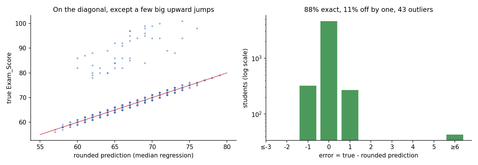
Left: true score against the rounded prediction; almost all points lie on the diagonal, but about 40 students score 10 to 30 points higher than predicted. Right: distribution of the errors on a log scale: 88 percent exact, 11 percent off by one, and 43 outliers far above.

About 0.8 % of the students have scores 10 to 30 points above what the formula predicts, scattered at random. Least squares, which penalises squared errors, tilts the whole fitted plane upward to reduce these huge errors, and so makes small errors on everybody else. Median (L1) regression, fitted with QuantileRegressor(quantile=0.5, alpha=0), treats an outlier like any other point and leaves the plane where the bulk of the data is. Its rounded predictions are exactly right for 88 % of students (78 % for least squares), and the CV MAE drops to 0.295.

Can we do better on the outliers? No feature predicts them (they look like random jumps added by the generator), and they account for 62 % of our remaining total error. Since the conditional median of their score is still on the plane, predicting the plane is the MAE-optimal choice.

The full solution

Subtasks 1 to 4 as above.
Map each ordered category to 0, 1, 2 (Yes = 1, Private = 1, Female = 1), fill the few missing values with the training median.
Fit a median regression (L1 loss, no regularisation) on all 19 features.
Round the predictions to the nearest integer.

model = QuantileRegressor(quantile=0.5, alpha=0, solver="highs").fit(X, y)
pred = np.round(model.predict(X_test))

Results

5-fold cross-validated MAE on the 5,285 training students:

approach	MAE	MAE with rounded predictions
constant median	2.832	2.832
gradient boosting	0.880	0.840
least-squares regression	0.498	0.396
least squares, one-hot encoding with a "missing" category	0.506	0.406
median regression, one-hot encoding	0.454	0.300
median regression, ordinal encoding (final)	0.454	0.295

Ordinal and one-hot encodings give the same result, which confirms that the effect of each Low/Medium/High column is really linear in the level. The two decisive steps are both about the metric: L1 loss (0.396 $\to$ 0.295 once rounded) and rounding (0.454 $\to$ 0.295).

What to remember

Match the loss to the metric: MAE is minimised by the median, so fit with an L1 / quantile loss when the evaluation is MAE, especially with outliers.
Exploit the type of the target: an integer target rewards rounding, a bounded target rewards clipping.
Ordered categories can be encoded as numbers when their effect is monotone and evenly spaced; check by comparing with one-hot encoding.
Do not reach for boosting by reflex: when a linear model already leaves tiny residuals, the truth is close to linear, and trees can only approximate it.
Look at the error distribution, not only its mean: here 62 % of the remaining error came from 43 unpredictable students, which tells you to stop tuning.

"""Exam score prediction (ROAI 2025, OJIA simulation 3, problem 2).

Subtasks 1-4: per-student statistics. Subtask 5: regress Exam_Score (integer), scored by MAE.

Key findings: the score is an (almost) exact linear function of the features, rounded to an integer,
plus a few rare large positive jumps. So: ordinal-encode the Low/Medium/High-style columns, fit a
median (L1) regression, which is the right estimator for MAE and ignores the outliers, and ROUND the
predictions to integers (the target is an integer): 0.50 -> 0.29 MAE.

Run from the folder holding train_data.csv and test_data.csv. 5-fold CV on train (test labels private).
"""
import numpy as np
import pandas as pd
from sklearn.linear_model import LinearRegression, QuantileRegressor
from sklearn.ensemble import HistGradientBoostingRegressor
from sklearn.metrics import mean_absolute_error
from sklearn.model_selection import KFold, cross_val_predict

tr = pd.read_csv("train_data.csv"); te = pd.read_csv("test_data.csv")
y = tr["Exam_Score"].values

# ---------------- subtasks 1 to 4 ----------------
t1 = (te["Hours_Studied"] - tr["Hours_Studied"].mean()).abs()
t2 = te["Sleep_Hours"] < 7
prev = np.sort(tr["Previous_Scores"].values)
t3 = len(prev) - np.searchsorted(prev, te["Previous_Scores"].values, side="left")   # train scores >= student's
t4 = te["Motivation_Level"].map(tr["Motivation_Level"].value_counts()).fillna(0).astype(int)

# ---------------- subtask 5 ----------------
ORDER = {"Low": 0, "Medium": 1, "High": 2, "Negative": 0, "Neutral": 1, "Positive": 2, "Near": 0, "Moderate": 1,
         "Far": 2, "High School": 0, "College": 1, "Postgraduate": 2, "No": 0, "Yes": 1, "Public": 0, "Private": 1,
         "Male": 0, "Female": 1}
CAT = [c for c in tr.columns if not pd.api.types.is_numeric_dtype(tr[c])]


def encode(d):
    X = d.drop(columns=["ID", "Exam_Score"], errors="ignore").copy()
    for c in CAT: X[c] = X[c].map(ORDER)
    return X


X, Xt = encode(tr), encode(te)
fill = X.median()                     # 3 ordinal columns have ~1 % missing values
X, Xt = X.fillna(fill), Xt.fillna(fill)
lad = lambda: QuantileRegressor(quantile=0.5, alpha=0, solver="highs")      # median regression = L1 loss

kf = KFold(5, shuffle=True, random_state=0)
print(f"constant median           MAE {mean_absolute_error(y, np.full(len(y), np.median(y))):.4f}")
for name, model in [("gradient boosting", HistGradientBoostingRegressor(random_state=0)),
                    ("least squares", LinearRegression()), ("median regression", lad())]:
    p = cross_val_predict(model, X, y, cv=kf)
    print(f"{name:25s} MAE {mean_absolute_error(y, p):.4f}   rounded to integers {mean_absolute_error(y, np.round(p)):.4f}")

pred = np.round(lad().fit(X, y).predict(Xt))
rows = []
for k, values in enumerate([t1, t2, t3, t4, pred], start=1):
    rows += [(k, i, v) for i, v in zip(te["ID"], values)]
pd.DataFrame(rows, columns=["subtaskID", "datapointID", "answer"]).to_csv("submission.csv", index=False)
print("wrote submission.csv")

Predicția scorului la examen