Problema Admiterii la un liceu de elită

The problem in brief

An elite high school admits or rejects candidates, and you get the file of 270 past candidates with their gender, county, four grades and the decision. The grades are the school's own admission test (NT), the national evaluation (MEV), the middle-school mathematics average (MATE) and the overall middle-school average (MGIM). For 180 test candidates you must output three things: the difference NT - MEV (20 points), each candidate's rank by MEV (20 points) and a prediction of the decision (60 points). The data and statement come from the public mirror of the ROAI 2025 rounds (github.com/jaredliw/ioai-tsp-2025); the test labels are private, so the prediction subtask is evaluated by cross-validation.

How you are scored

Subtasks 1 and 2 are checked row by row. Subtask 3 uses accuracy, the share of test candidates whose decision you predict correctly:

$$\text{accuracy} = \frac{1}{n}\sum_{i=1}^{n} \mathbf 1\left[\hat y_i = y_i\right],$$

with a maximum of 60 points (Nitro task configuration: metric Accuracy, maximum 60). Submitting the sample file earns 5 points. No threshold, leaderboard or editorial for this round is public, so there is no published target.

The two warm-up subtasks

Subtask 1. NT - MEV with two decimals. The only trap is floating point: $9.52 - 6.24$ is stored as $3.2799999\ldots$, so round explicitly (round(2)) and print with two decimals.

Subtask 2. The rank of each test candidate by MEV, best grade first. Two details matter. First, the ranking is computed inside the test set (it is a property of the 180 candidates you are given, not of the training file). Second, the statement asks for distinct integers, yet 38 test candidates share their MEV with someone else, so a tie-breaking rule is needed. The natural one is the order of appearance in the file, which is what a stable sort gives:

t2 = te.MEV.rank(ascending=False, method="first").astype(int)

The statement does not say how ties are broken, so a few rows of this subtask depend on that convention.

First look at the data

Plot the decision against each grade and the picture is immediate: every admitted candidate has NT above 6.9 and every rejected one below 7.5. The admission test almost decides alone. The other grades only matter for the few candidates in the narrow band where NT lies between 6.9 and 7.5. Gender (28 % against 25 % admitted) and county (42 different values for 270 rows) carry no information, and id is just a counter.

There is a second, more surprising finding: 111 of the 180 test candidates are also in the training file, with the same id, gender, county and all four grades, and with their decision. Only 69 test candidates are genuinely new. A careful contestant should notice this (a simple merge on the grades finds it) because it means that 62 % of subtask 3 is answered by a lookup. Our model reproduces every training label anyway, so the lookup changes nothing here, but in other problems such a leak can be worth many points, and it also tells you that a "test score" computed on such rows says nothing about generalisation.

A first baseline

The one-feature rule "admitted if NT is above a threshold" (a depth-1 decision tree) already reaches 97.7 % cross-validated accuracy (5-fold, repeated 5 times). A standardised logistic regression on the four grades with default regularisation ($C = 1$) reaches 98.5 %.

The key idea

Real admission decisions are rarely learned patterns: they apply a published formula. The school computes a weighted average of the grades and admits everyone above a cut-off (or the best $k$ candidates, which amounts to the same thing for a fixed year). If that is the case here, the two classes are separated by a hyperplane

$$w_1\,\mathrm{NT} + w_2\,\mathrm{MEV} + w_3\,\mathrm{MATE} + w_4\,\mathrm{MGIM} \ge \theta ,$$

and the right model is a linear classifier fitted with little or no regularisation. Checking the hypothesis is easy: fit a linear model with a very large $C$ and look at the training accuracy. It is exactly 100 %. The data are linearly separable.

Separable data has a consequence worth understanding. Logistic regression with a weak penalty pushes its weights towards infinity (the likelihood keeps growing as the margin is scaled up), and its default $C = 1$ shrinks the weights so much that the boundary tilts and misclassifies a few borderline candidates. That is why accuracy rises from 98.5 % to 99.4 % when $C$ goes from 1 to 1000. The cleanest tool for separable data is the maximum-margin linear classifier, a linear SVM with a large $C$: among all separating hyperplanes it picks the one farthest from both classes. Rescaled so that the weights sum to 1, it finds

$$0.769\,\mathrm{NT} + 0.169\,\mathrm{MEV} - 0.019\,\mathrm{MATE} + 0.080\,\mathrm{MGIM} \ge 7.32 .$$

This reads like an admission formula: about three quarters for the school's own test, a quarter for the earlier results, and essentially nothing for the mathematics average (its weight is tiny and slightly negative, which is noise). Several "round" formulas also separate the training set perfectly, for instance $0.75\,\mathrm{NT} + 0.15\,\mathrm{MEV} + 0.10\,\mathrm{MGIM}$, or $0.75\,\mathrm{NT} + 0.25\,(0.8\,\mathrm{MEV} + 0.2\,\mathrm{MGIM})$, which uses the 80/20 weighting of the Romanian admission average. With only 270 rows we cannot tell which one the organisers used.

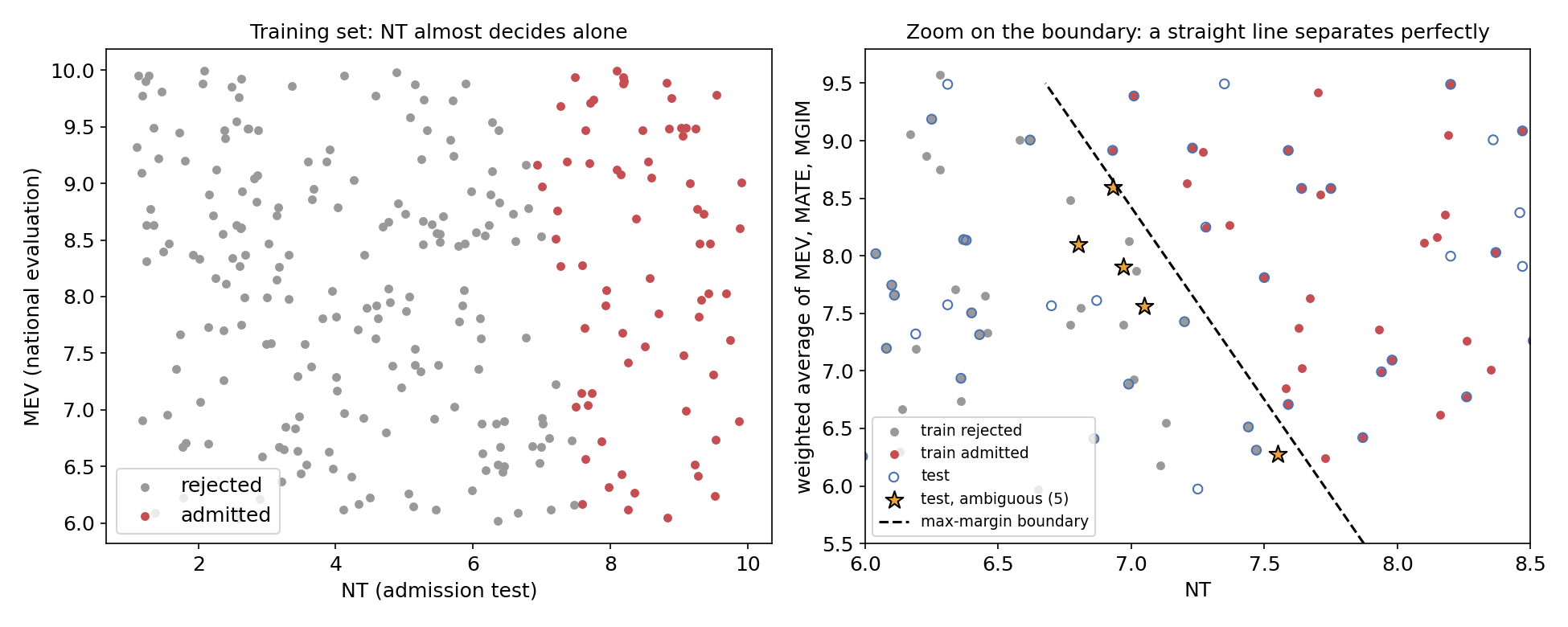
How much does that uncertainty cost? We enumerated every weight vector on a grid of step 0.0125 (weights summing to 1) that separates the training data, 215 of them, and applied each to the test set with its mid-gap threshold. They agree on 175 of the 180 test candidates. The five others (all among the 69 new candidates) sit in the thin wedge where the possible boundaries cross, and all five are predicted "rejected" by the max-margin SVM and by most of the separating formulas. In the worst case the accuracy is therefore $175/180 = 97.2\,\%$, and most likely it is 99 to 100 %.

The full solution

1. Drop id, gen and judet; keep the four grades.
2. Standardise the grades (the statement asks for it, and it makes the SVM's penalty treat the four grades alike).
3. Fit a linear SVM with $C = 10^4$ (a hard margin in practice) and predict the 180 test candidates: 51 are admitted.
4. Write the three subtasks in the subtaskID, datapointID, answer format, with two decimals for subtask 1 and integers elsewhere.

model = make_pipeline(StandardScaler(), SVC(kernel="linear", C=1e4))
model.fit(tr[["NT", "MEV", "MATE", "MGIM"]], y)
t3 = model.predict(te[["NT", "MEV", "MATE", "MGIM"]])

Results

Subtask 3, 5-fold cross-validation repeated 5 times on the training set (the test labels are private):

approach	CV accuracy
sample output	5 points by rule
threshold on NT only (depth-1 tree)	0.977
logistic regression on the 4 grades, $C = 1$	0.985
logistic regression, $C = 1000$	0.994
linear SVM, $C = 10^4$ (final)	0.992
training accuracy of either linear model	1.000

The two weakly regularised models make identical test predictions. The remaining cross-validation errors come from folds where the few borderline candidates are held out, so the boundary has a little less information; on the full training set the boundary is pinned down by those very candidates. Subtasks 1 and 2 are deterministic (40 points), with the tie-breaking convention of subtask 2 as the only open point.

What to remember

• When a label comes from a rule, look for the rule. Admissions, tax brackets, grading schemes are thresholds on weighted sums; a training accuracy of exactly 100 % with a linear model is the signature, and the fitted weights then read like the formula.
• Regularisation is a prior, and here the prior was wrong. On separable data a strong penalty tilts the boundary; a large $C$ or a max-margin SVM respects the separation.
• Measure what you cannot know. Enumerating all the rules consistent with the training data shows which test rows are truly uncertain (5 of 180), which turns a vague worry into a bound on the score.
• Always check train/test overlap. A merge on the features revealed that 111 test candidates were copied from the training file; in other problems such a leak can decide the ranking, and it always inflates any test-based estimate.
• Exact subtasks have exact traps. Round floating-point differences explicitly, compute ranks inside the right set, and break ties with a stated rule.