IOAI Training: Learn AI by solving problems

The problem in brief

You get 800 houses described by their area, number of bedrooms and bathrooms, year built, lot size, garage size, neighbourhood quality and a few derived ratios, plus five odd "sensor" columns (orientation angle, street alignment offset, solar exposure, magnetic field strength, vibration level). Four warm-up subtasks ask for simple per-house computations on the 200 test houses; the main subtask asks for a regression model of the house price, scored by mean absolute error.

How you are scored

Subtasks 1 to 4 are worth 10 points each, subtask 5 is worth 60. For subtask 5 the metric is

\text{MAE} = \frac{1}{n}\sum_{i=1}^{n}\lvert y_i - \hat y_i\rvert ,

"as low as possible". The statement gives no threshold or point formula for it, and we found no public leaderboard, so there is no target to compare with: we report the 5-fold cross-validated MAE on the training set (the test prices are private).

Subtasks 1 to 4

Pure column arithmetic, one value per test house:

subtask	formula
1	`Square_Footage + Garage_Size + Lot_Size`
2	`Garage_Size / Total_Rooms`
3	`(Solar_Exposure_Index - Vibration_Level) / Magnetic_Field_Strength`
4	`abs(Square_Footage - mean of Square_Footage over the TRAINING set)`

The only traps: the mean in subtask 4 comes from the training file, not the test file, and the units of subtask 1 are absurd (square feet plus a garage size in cars plus a lot size in acres): compute what is asked, not what makes physical sense. There are no missing values and no zero denominators.

First look at the data

The correlations with the price are revealing: Footage_to_Lot_Ratio (area divided by lot size) has 0.92, Square_Footage 0.75, Lot_Size $-0.42$ , and the year, bedrooms or neighbourhood quality almost nothing. The five sensor columns are uniformly spread between 0 and 360 and uncorrelated with everything: they are distractors.

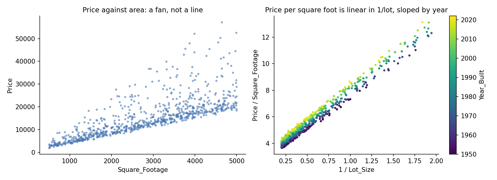
Left: price against area, a fan of points that widens as the area grows. Right: price per square foot against one over the lot size, coloured by construction year: the points lie on a narrow straight band, newer houses slightly higher.

The left plot is a fan, not a line: the price grows with the area, but by an amount that differs from house to house. Dividing by the area (right plot) collapses the fan: the price per square foot is almost exactly a straight line in $1/\text{lot size}$ , shifted up a little for newer houses. In other words, the price is close to

\text{Price} \approx \text{area} \times \Big(a + \frac{b}{\text{lot}} + c\cdot\text{year} + d\cdot\frac{\text{year}}{\text{lot}} + \dots\Big),

a product of features, which is exactly what a linear model on the raw columns cannot represent.

A first baseline

Predicting the median price: MAE 6,417.
Linear regression on all 17 raw columns: MAE 264. It gets far because Footage_to_Lot_Ratio is already one of the products we need.
Gradient boosting on the raw columns: MAE 488, worse than linear. With 800 houses, trees approximate a smooth multiplicative surface with many small steps and cannot extrapolate along it.

The key idea

Give the linear model the products it needs. If the price is area times a linear function of other features, then expanding the product gives terms like area $\times$ year, area $/$ lot, area $\times$ bedrooms: create those columns and the model becomes linear again in its inputs. With 16 such features (area, area/lot, area $\times$ year, area/lot $\times$ year, area times bedrooms, bathrooms, garage and quality, area $^2$ , plus the plain columns), linear regression reaches MAE 69, four times better than with the raw columns.

Then let trees fix what is left. The residuals of this model are small and no longer have an obvious structure; a gradient-boosting model trained on the residuals (with the raw columns as input) captures the remaining interactions and brings the MAE to 43. This "linear model for the big smooth structure, trees for the leftovers" combination is a classical and very effective form of stacking: each model does what it is good at.

How do we find which products matter? We did not guess them all at once: we fitted the price per square foot (the right plot) with a linear model, looked at which features its residuals still correlated with (area, the ratio), added the corresponding products, and checked each addition by cross-validation. Dropping area/lot, area × year or area/lot × year each costs 70 to 100 points of MAE; most others matter little.

The full solution

Subtasks 1 to 4 as above.
Build the product features.
Fit LinearRegression on them.
Fit HistGradientBoostingRegressor on the residuals, with the raw columns as inputs.
Predict: linear prediction + boosted residual correction.

self.lin = LinearRegression().fit(products(d), y)
self.gb  = HistGradientBoostingRegressor().fit(d[RAW], y - self.lin.predict(products(d)))
pred     = self.lin.predict(products(d)) + self.gb.predict(d[RAW])

Results

5-fold cross-validated MAE on the 800 training houses:

approach	CV MAE
constant median	6,417
gradient boosting, raw columns	488
linear regression, raw columns	264
linear regression, raw columns, median (L1) loss	257
log-price linear model with log area and log lot	133
price-per-square-foot linear model	178
linear regression on product features	69
+ gradient boosting on its residuals (final)	43

The typical price is 15,000, so the final error is about 0.3 % of the price. Changing the loss (median regression) barely helped: the problem was the form of the model, not its robustness.

What to remember

Plot the target against the main feature. A fan shape means a multiplicative effect: divide by the feature (here, price per square foot) and look again.
Linear models are only linear in their features. Products and ratios turn a curved relation into a linear one; the given Footage_to_Lot_Ratio was a hint.
Trees are not always the best tool on small tabular data: with 800 rows and a smooth structure, they lost to a well-specified linear model, and won only as a residual corrector.
Stacking by residuals: fit the simple global structure first, then let a flexible model learn what remains.
Ignore distractor columns after checking them: the sensor-like columns had zero correlation with the price and with the residuals.

"""House price prediction (ROAI 2025, OJIA simulation 2, problem 2).

Subtasks 1-4: per-house arithmetic on test_data.csv. Subtask 5: regress Price (MAE).

Key finding: the price is (almost) the house area times a "price per square foot" that depends on
1/Lot_Size, the year, bedrooms and bathrooms. A linear model on raw columns cannot express such
products (CV MAE 264); a linear model on the product features does (69), and gradient boosting on its
residuals mops up the rest (44). The sensor-like columns (angles, magnetic field...) are pure noise.

Run from the folder holding train_data.csv and test_data.csv. 5-fold CV on train (test labels private).
"""
import numpy as np
import pandas as pd
from sklearn.ensemble import HistGradientBoostingRegressor
from sklearn.linear_model import LinearRegression
from sklearn.metrics import mean_absolute_error
from sklearn.model_selection import KFold, cross_val_predict

tr = pd.read_csv("train_data.csv"); te = pd.read_csv("test_data.csv")
y = tr["Price"].values
RAW = [c for c in tr.columns if c not in ["ID", "Price"]]

# ---------------- subtasks 1 to 4 (one value per test house) ----------------
task1 = te["Square_Footage"] + te["Garage_Size"] + te["Lot_Size"]
task2 = te["Garage_Size"] / te["Total_Rooms"]
task3 = (te["Solar_Exposure_Index"] - te["Vibration_Level"]) / te["Magnetic_Field_Strength"]
task4 = (te["Square_Footage"] - tr["Square_Footage"].mean()).abs()      # mean from TRAIN


# ---------------- subtask 5 ----------------
def products(d):
    s, lot, yr = d["Square_Footage"], d["Lot_Size"], d["Year_Built"]
    return pd.DataFrame({
        "sqft": s, "sqft_over_lot": s / lot, "sqft_x_year": s * yr, "sqft_over_lot_x_year": s / lot * yr,
        "sqft_x_bed": s * d["Num_Bedrooms"], "sqft_x_bath": s * d["Num_Bathrooms"], "sqft_x_garage": s * d["Garage_Size"],
        "sqft_x_quality": s * d["Neighborhood_Quality"], "sqft2": s ** 2, "year": yr, "lot": lot, "lot2": lot ** 2,
        "bed": d["Num_Bedrooms"], "bath": d["Num_Bathrooms"], "garage": d["Garage_Size"], "quality": d["Neighborhood_Quality"]})


class LinearPlusBoost:
    """Linear model on product features, then gradient boosting on its residuals (raw columns)."""

    def fit(self, d, y):
        self.lin = LinearRegression().fit(products(d), y)
        self.gb = HistGradientBoostingRegressor(random_state=0).fit(d[RAW], y - self.lin.predict(products(d)))
        return self

    def predict(self, d):
        return self.lin.predict(products(d)) + self.gb.predict(d[RAW])


kf = KFold(5, shuffle=True, random_state=0)
cv = lambda make: mean_absolute_error(y, np.concatenate(
    [make().fit(tr.iloc[a], y[a]).predict(tr.iloc[b]) for a, b in kf.split(tr)])[np.argsort(np.concatenate([b for _, b in kf.split(tr)]))])
print(f"constant median          CV MAE {mean_absolute_error(y, np.full(len(y), np.median(y))):8.1f}")
print(f"linear, raw columns      CV MAE {mean_absolute_error(y, cross_val_predict(LinearRegression(), tr[RAW], y, cv=kf)):8.1f}")
print(f"boosting, raw columns    CV MAE {mean_absolute_error(y, cross_val_predict(HistGradientBoostingRegressor(random_state=0), tr[RAW], y, cv=kf)):8.1f}")
print(f"linear, product features CV MAE {mean_absolute_error(y, cross_val_predict(LinearRegression(), products(tr), y, cv=kf)):8.1f}")
print(f"linear products + boost  CV MAE {cv(LinearPlusBoost):8.1f}")

price = LinearPlusBoost().fit(tr, y).predict(te)
rows = []
for k, values in enumerate([task1, task2, task3, task4, price], start=1):
    rows += [(k, i, float(v)) for i, v in zip(te["ID"], values)]
pd.DataFrame(rows, columns=["subtaskID", "datapointID", "answer"]).to_csv("submission.csv", index=False)
print("wrote submission.csv")

Predicția prețului unei case