Robots in the Maze

The problem in brief

A robotics lab logs one row per experiment: the arena (desert, forest, ice, urban), the weather, and about twenty numbers measured during the run, such as average speed, distance, collisions, items picked up, pauses, turn rate or how consistently the robot patrols. Each robot follows one of four strategies: explorer (visit as many places as possible), collector (pick up items), guardian (patrol the same regions) and sprinter (go fast). You get 1 200 labelled experiments in train.csv and 400 unlabelled ones in test.csv. Four warm-up questions ask for simple statistics of the training table, and the main task asks you to predict the strategy of every test robot.

How you are scored

Tasks 1 to 4 (50 points in total) are checked by exact equality with the value computed from train.csv. Task 5 (50 points) uses the macro F1-score over the $K = 4$ strategies. For a class $c$ with precision $P_c$ and recall $R_c$:

$$F1_c = \frac{2\,P_c\,R_c}{P_c + R_c}, \qquad \text{Macro-F1} = \frac{1}{4}\sum_{c=1}^{4} F1_c .$$

The points for task 5 are $50 \times \text{Macro-F1}$, capped at 50 as soon as Macro-F1 reaches 0.93. So the target is clear: 0.93 macro F1 gives full marks, and nothing above it counts.

The test labels are private, so all task 5 scores below come from cross-validation on the training set.

First look at the data

Tasks 1 to 4 are one line of pandas each:

task	code	answer
1. number of arena types	train.arena_type.nunique()	4
2. maximum average speed	train.avg_speed_mps.max()	2.641200394995685
3. most frequent arena	train.arena_type.value_counts().idxmax()	forest (414 rows)
4. maximum items collected	train.items_collected.max()	22

The only trap is task 2. Grading is by exact equality, so do not round the maximum speed: the example file shows 4.31, but the true value has 16 significant digits, and writing 2.64 would lose 15 points. Print it with repr() or let pandas write the float to the CSV.

For task 5, the table is clean: no missing values, classes reasonably balanced (352 explorers, 307 collectors, 304 sprinters, 237 guardians). A few columns are clipped at a bound (99 rows have detour_index exactly $-10$, 185 rows have efficiency_score exactly 10). That is a sign the data is synthetic: every value looks like a draw from a distribution that depends on the strategy, plus noise, then clipped. Some pairs of columns are strongly tied (speed and distance correlate at 0.93, items collected and pickup efficiency at 0.93), as you would expect physically.

The most useful look is the average of each feature per strategy, measured in standard deviations from the overall mean:

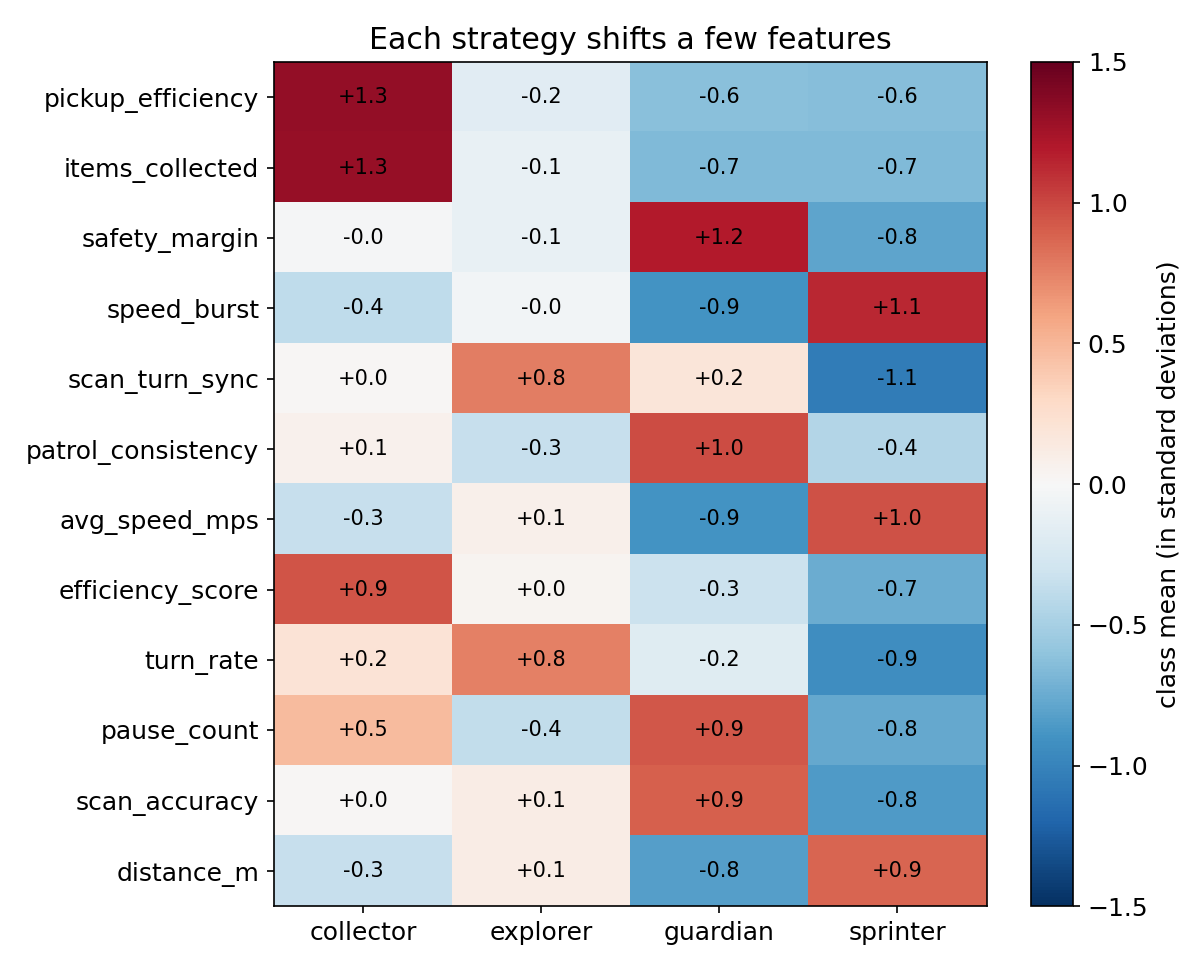
Every strategy has a clear signature that matches its description. Collectors pick up many items (+1.3 std). Guardians are slow, careful (large safety margin, many pauses, accurate scans) and consistent patrollers. Sprinters are fast, with big speed bursts, long distances and few turns. Explorers are the middle class: they turn a lot and synchronise scans with turns, but on most features they sit near the average. Expect the explorers to be the hardest class to recognise.

A first baseline

Always start with the trivial predictor: answering "explorer" for every robot gives macro F1 0.113, because three of the four classes get an F1 of zero. Then try the usual tabular workhorse, a random forest with 500 trees on all features (arena and weather one-hot encoded). With 5-fold cross-validation repeated 3 times it reaches 0.913 macro F1. Gradient boosting does about the same (0.918). That is close, but still under the 0.93 threshold, so around 46 points instead of 50.

The key idea

Look at the shape of the classes before reaching for the most powerful model. The profile figure suggests that each strategy simply shifts the mean of a handful of features, with roughly the same spread in every class. If each class $c$ is a Gaussian cloud with mean $\mu_c$ and a covariance $\Sigma$ shared by all classes, the Bayes-optimal classifier has a closed form. Taking the log of $p(x \mid c)\,\pi_c$ and dropping the terms that do not depend on $c$ gives a score that is linear in $x$:

$$\delta_c(x) = x^\top \Sigma^{-1}\mu_c \;-\; \tfrac12\,\mu_c^\top \Sigma^{-1}\mu_c \;+\; \log \pi_c ,$$

and we predict the class with the largest $\delta_c(x)$. The quadratic term $x^\top\Sigma^{-1}x$ is the same for every class, so it cancels: the boundaries between classes are hyperplanes. This model is Linear Discriminant Analysis (LDA). It estimates only the four means and one pooled covariance matrix, about 300 numbers in total, so it is very stable with 1 200 rows.

A tree ensemble, by contrast, has to approximate each oblique hyperplane with a staircase of axis-aligned splits, and with 1 200 noisy rows the staircase is coarse. That is exactly why the forest, usually stronger on tabular data, loses here. The data was generated in a way that favours a linear boundary, and a linear model matches that structure.

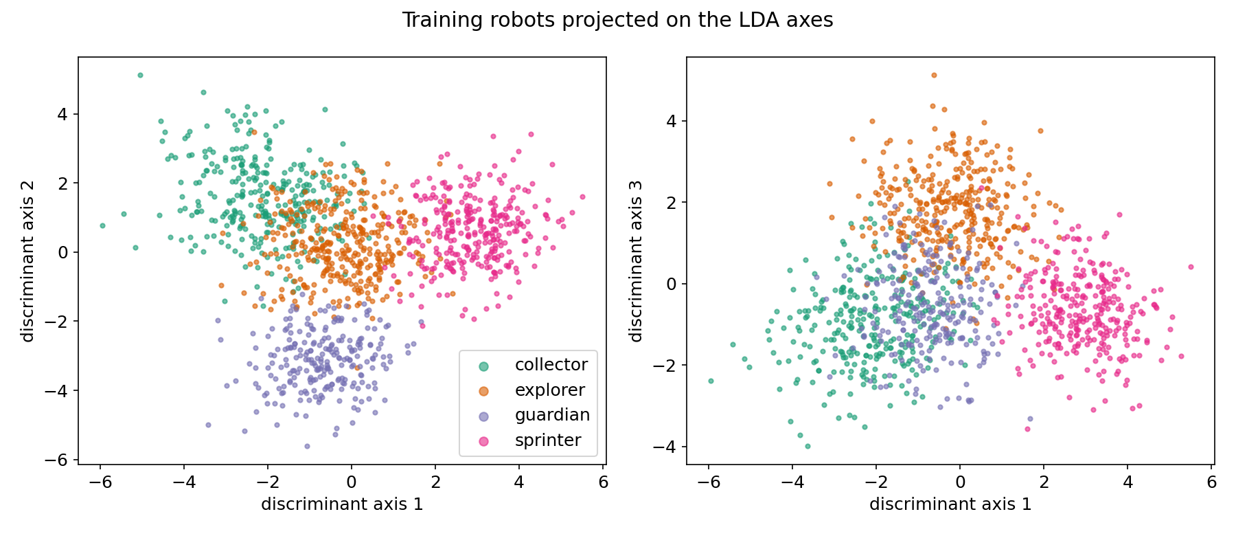
The figure below projects the training robots on the three LDA directions (the directions that best separate the class means relative to the shared spread). Guardians and sprinters form clean, separate clouds. Collectors and explorers touch each other, and explorers sit in the middle of everything, as the profiles predicted.

The full solution

1. Features. Drop robot_id, one-hot encode arena_type and weather, keep all numeric columns as they are. No feature engineering is needed: adding flags for the clipped values did not help (0.939).
2. Model. Standardise, then fit LinearDiscriminantAnalysis(). Standardising does not change LDA's predictions, but it makes the coefficients comparable between features.
3. Validation. 5-fold stratified cross-validation repeated 3 times, scored with f1_score(average="macro"). The standard deviation over folds (about 0.015) tells you that differences of 0.003 between linear models are just noise.
4. Submission. Four GLOBAL rows for tasks 1 to 4 (full-precision speed), then one row per test robot with subtask 5.

X = pd.get_dummies(train.drop(columns=["robot_id", "strategy_label"]),
                   columns=["arena_type", "weather"]).astype(float)
model = make_pipeline(StandardScaler(), LinearDiscriminantAnalysis())
model.fit(X, train["strategy_label"])

The cross-validated confusion matrix of LDA confirms the picture. Guardians (F1 0.962) and sprinters (0.969) are almost always right. The remaining errors are mostly collectors taken for explorers (23) and explorers taken for collectors or sprinters (13 and 11). Explorers have the lowest F1 (0.910), because a robot that explores a lot also collects some items and moves fairly fast: it shares a little of every other signature.

Results

Task 5 scores: macro F1, 5-fold stratified CV repeated 3 times on the 1 200 training rows (the test labels are private).

approach	macro F1 (CV)	task 5 points
always "explorer"	0.113	5.7
random forest, 500 trees	0.913 ± 0.019	45.7
gradient boosting (HistGradientBoosting)	0.918	45.9
RBF SVM, C = 1	0.936 ± 0.013	50
logistic regression, C = 0.3	0.941 ± 0.015	50
logistic regression + clipping flags	0.939 ± 0.014	50
linear SVM	0.945 ± 0.014	50
LDA (final)	0.944 ± 0.016	50

With tasks 1 to 4 exact, the expected total is the full 100 points: the final model clears the 0.93 cap by about one standard deviation of the CV estimate.

What to remember

• Exact-match questions punish rounding. When a grader compares values by equality, print floats at full precision (repr), never the two decimals shown in an example.
• Look at class profiles first. A table of class means in standard deviations tells you in one glance which features matter and which class will be hard (the one with no strong signature).
• Match the model to the structure of the data. When classes are shifted Gaussian clouds, the optimal boundary is linear, and LDA or logistic regression beats random forests and boosting, which must build oblique boundaries from axis-aligned steps.
• Know your threshold. Above 0.93 extra macro F1 earns nothing, so a simple, stable model with a safety margin is better than a fragile one tuned to the third decimal.
• Read CV noise before comparing models. With a fold-to-fold standard deviation around 0.015, logistic regression, LDA and a linear SVM are tied; pick the simplest.