IOAI Training: Learn AI by solving problems

The problem in brief

Each image is a 168 x 168 black canvas on which between 2 and 5 small garments from Fashion-MNIST (T-shirt, trouser, pullover, dress, coat, sandal, shirt, sneaker, bag, ankle boot) have been pasted at random places. You must say, for each of the 10 garment types, whether it appears at least once. This is multi-label classification: several answers can be true at once, unlike ordinary classification where exactly one class wins. You get 6 318 training images and 702 validation images; the 780 test images are hidden on the contest platform, which allows pretrained ResNets from torchvision and limits the evaluation to 2.5 minutes on a GPU.

The test set is private, so all scores below are on the official validation set, which the organisers say was built exactly like the test set. We never tuned anything on it.

How you are scored

For each class $c$ , the F1-score compares the predicted and true presence over all images; the task metric is their average (macro F1):

F1_c = \frac{2\,TP_c}{2\,TP_c + FP_c + FN_c}, \qquad \text{F1} = \frac{1}{10}\sum_{c} F1_c .

Points follow a linear scale between two thresholds published in the statement: 0 points at F1 $\le 0.57$ , 100 points at F1 $\ge 0.87$ , and $100\,(F1 - 0.57)/0.30$ in between.

The lower threshold is not arbitrary. Each garment type is present in about 37 % of the images, so the naive solution that answers "every garment is present" has recall 1 and precision 0.37 for every class, hence F1 $= 2 \cdot 0.37/(1.37) \approx 0.54$ . Anything at or below 0.57 is no better than that.

First look at the data

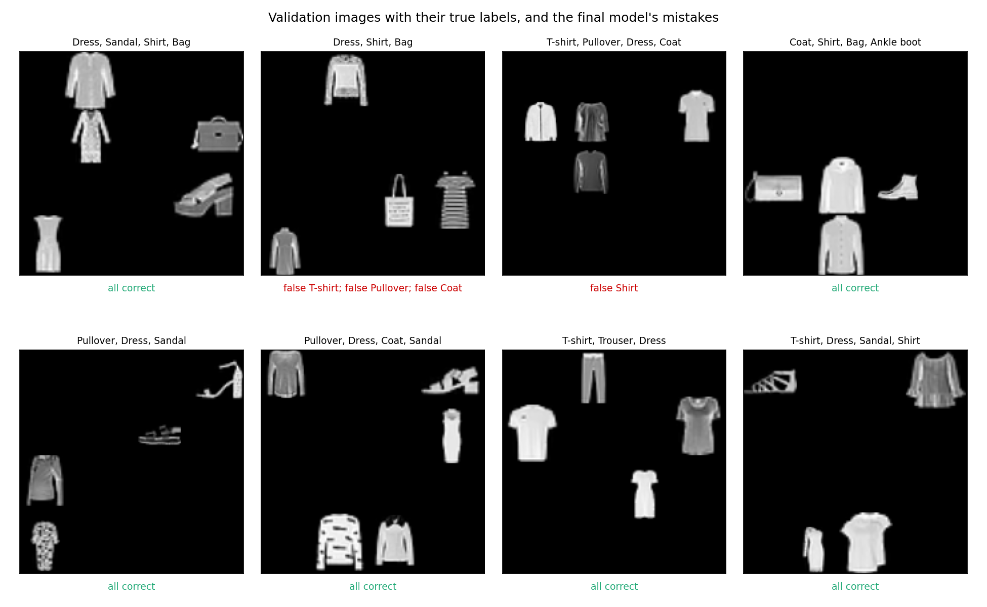
Validation images with their labels

Every class appears in 35 to 39 % of the images: the classes are balanced, so there is no imbalance trick to play.
Most images hold 3 or 4 garments, each about 20 to 40 pixels wide, anywhere on the canvas, sometimes touching the border. The same garment type can appear twice.
The hard part is inherited from Fashion-MNIST: shirt, T-shirt, pullover and coat look alike at this resolution. Footwear (sandal, sneaker, ankle boot), trousers and bags are easy.

A first baseline

The "everything is present" answer scores 0.545 (0 points). A pixel-based model does even worse: a one-vs-rest logistic regression on the image downsampled to 42 x 42 gets 0.423. That is a useful lesson. A linear model on pixels learns "a bright blob at this location means a trouser", but a trouser can be anywhere, so the weights for every location get averaged into mush. What we need is a detector that recognises a garment wherever it is.

The key idea

A convolutional network followed by global pooling is a "find it anywhere" detector, and one sigmoid per class turns it into ten independent yes/no questions.

Convolutions are translation-equivariant. The same filters slide over the whole image, so a trouser produces the same activations at the top-left as at the bottom-right, just shifted.
Global pooling removes the position. After four blocks of convolutions and pooling, the network has a 10 x 10 map of 256 features. Taking the maximum (or the mean) of each feature over the whole map gives a 256-number summary that no longer depends on where the garments were. Max pooling matches the question exactly ("is there a trouser somewhere?"), while average pooling counts how much of it there is; in our runs both work equally well (0.924 and 0.926), because the final linear layer and the threshold can absorb the difference.
Sigmoid + binary cross-entropy, not softmax. A softmax makes the classes compete for a probability mass of 1, which is wrong when 4 garments are present. With 10 sigmoids, each output answers its own question:

\mathcal L = -\frac{1}{10}\sum_{c=1}^{10} \Big[ y_c \log \sigma(z_c) + (1-y_c)\log\big(1-\sigma(z_c)\big) \Big].

We predict "present" when $\sigma(z_c) > 0.5$ .

The full solution

Scale pixels to $[0, 1]$ . Hold out 600 training images (only to test per-class thresholds, see below).
Network trained from scratch: four blocks of two 3 x 3 convolutions with batch normalisation and ReLU, each followed by 2 x 2 max-pooling (32, 64, 128, 256 channels; 168 to 10 pixels), global max pooling, one linear layer to 10 logits. About 1.2 M parameters.
Augmentation: random horizontal flip and random shift of up to 12 pixels (with wrap-around). Both preserve the labels.
30 epochs of AdamW (learning rate $10^{-3}$ with a one-cycle schedule, weight decay $10^{-4}$ , batch 64): about 10 minutes on an Apple GPU, around a minute or two on a contest GPU. Prediction averages the image and its mirror.

f = self.features(x)          # (B, 256, 10, 10)
z = self.head(f.amax((2, 3))) # "is feature k present anywhere?" -> 10 logits
loss = F.binary_cross_entropy_with_logits(z, y)

The pretrained ResNets allowed by the statement were not needed: the garments are tiny grey-scale icons, very different from ImageNet photos, and a small network trained from scratch already clears the 100-point threshold by a wide margin.

Thresholds. Tuning one threshold per class on the 600 held-out training images changed almost nothing (0.923 against 0.924 at 0.5): when classes are balanced and the model is well calibrated, 0.5 is already close to optimal for F1.

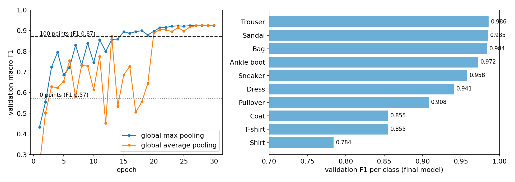
Validation macro F1 during training, and per-class F1 of the final model

The per-class scores tell the expected story: trousers, sandals and bags are near 0.99, while shirt (0.78), T-shirt and coat (0.86) are the weak spots, because at 28 x 28 pixels a shirt, a pullover, a coat and a T-shirt differ by a collar, a zip or the sleeve length. The same four classes are the classic confusions of single-label Fashion-MNIST.

Results

Official validation set (702 images); the test labels are private.

approach	val macro F1	points
answer "all 10 present" (statement's naive solution)	0.545	0
logistic regression on 42 x 42 pixels	0.423	0
CNN + global average pooling	0.926	100
CNN + global max pooling, threshold 0.5 (final)	0.924	100
same, per-class thresholds tuned on held-out training images	0.923	100

The final model reaches 0.924 macro F1 on validation, well above the 0.87 needed for full marks; since the test set is built the same way, the margin of 0.05 should be comfortable.

What to remember

Multi-label means one sigmoid per class, trained with binary cross-entropy; softmax would force the classes to compete.
"Is it anywhere in the image?" calls for convolutions plus global pooling, which make the answer independent of position. A linear model on pixels cannot do this and scores below the trivial baseline.
Compute the trivial baseline of your metric. "Everything present" gives F1 0.54 here, which explains the statement's 0-point threshold of 0.57.
Pretrained is not always necessary. For small synthetic icons, a compact CNN trained from scratch for 10 minutes beats the threshold easily.
Look at per-class scores. The average hides that shirt and T-shirt carry most of the remaining errors.

"""Multi-label classification (Polish OAI 2026, stage 1): which of 10 Fashion-MNIST garment types
appear in a 168x168 image holding 2 to 5 garments at random positions.  Metric: macro F1
(100 points at F1 >= 0.87).  The test set is hidden; we report the official validation set.

Model: a small VGG-style CNN trained from scratch with 10 sigmoid outputs (binary cross-entropy),
GLOBAL MAX POOLING over the final feature map ("is this garment anywhere?"), horizontal-flip and
shift augmentation, flip test-time averaging.  ~10 minutes on an Apple GPU for 30 epochs.
Usage: POOL=max python solution.py      (POOL=avg for the ablation)
Data: runway-mnist/{train,val}-{x,y}.npz from the statement notebook (Drive id 1oNAFYdJyCVe3Po90KLUPxAG9HGuL7NSw)
"""
import os, time, numpy as np, torch, torch.nn as nn, torch.nn.functional as F
from sklearn.metrics import f1_score
torch.set_num_threads(2); torch.manual_seed(42); np.random.seed(42)
DEV = "cuda" if torch.cuda.is_available() else ("mps" if torch.backends.mps.is_available() else "cpu")
POOL = os.environ.get("POOL", "max"); EPOCHS = 30

load = lambda f, k: np.load(f"runway-mnist/{f}.npz")[k]
X = torch.tensor(load("train-x", "images")).float().unsqueeze(1) / 255.; Y = torch.tensor(load("train-y", "labels")).float()
VX = torch.tensor(load("val-x", "images")).float().unsqueeze(1) / 255.; VY = load("val-y", "labels")
perm = torch.randperm(len(X)); hold, tr = perm[:600], perm[600:]     # 600 training images to tune thresholds


class Net(nn.Module):
    """4 blocks of two 3x3 convs + BN + ReLU + 2x2 max-pool: 168 -> 84 -> 42 -> 21 -> 10 pixels."""
    def __init__(self):
        super().__init__()
        c, layers = [1, 32, 64, 128, 256], []
        for a, b in zip(c, c[1:]):
            layers += [nn.Conv2d(a, b, 3, padding=1), nn.BatchNorm2d(b), nn.ReLU(),
                       nn.Conv2d(b, b, 3, padding=1), nn.BatchNorm2d(b), nn.ReLU(), nn.MaxPool2d(2)]
        self.features, self.head = nn.Sequential(*layers), nn.Linear(256, 10)

    def forward(self, x):
        f = self.features(x)                                    # (B, 256, 10, 10) feature map
        pooled = f.amax((2, 3)) if POOL == "max" else f.mean((2, 3))
        return self.head(pooled)                                # 10 independent logits


model = Net().to(DEV)
opt = torch.optim.AdamW(model.parameters(), lr=1e-3, weight_decay=1e-4)
sched = torch.optim.lr_scheduler.OneCycleLR(opt, max_lr=1e-3, total_steps=EPOCHS * (len(tr) // 64))


def augment(x):
    if np.random.rand() < .5: x = x.flip(3)                     # a mirrored garment is the same garment
    dx, dy = np.random.randint(-12, 13, 2)                      # garments can be anywhere
    return torch.roll(x, (int(dy), int(dx)), (2, 3))


@torch.no_grad()
def probs(x):
    model.eval(); out = []
    for i in range(0, len(x), 128):
        b = x[i:i + 128].to(DEV)
        out.append(((torch.sigmoid(model(b)) + torch.sigmoid(model(b.flip(3)))) / 2).cpu())
    model.train(); return torch.cat(out).numpy()


t0 = time.time()
for ep in range(EPOCHS):
    idx = tr[torch.randperm(len(tr))]
    for i in range(0, len(idx) - 63, 64):
        b = idx[i:i + 64]
        loss = F.binary_cross_entropy_with_logits(model(augment(X[b]).to(DEV)), Y[b].to(DEV))
        opt.zero_grad(); loss.backward(); opt.step(); sched.step()
    print(f"epoch {ep + 1}: val macro F1 @0.5 = {f1_score(VY, probs(VX) > 0.5, average='macro'):.4f} ({time.time() - t0:.0f}s)")

# optional per-class thresholds, tuned on the 600 held-out TRAINING images (never on val)
ph, yh = probs(X[hold]), Y[hold].numpy()
th = np.array([max(np.arange(.2, .8, .02), key=lambda t: f1_score(yh[:, c], ph[:, c] > t)) for c in range(10)])
pv = probs(VX)
f1 = f1_score(VY, pv > .5, average="macro")
print(f"val macro F1: {f1:.4f} at 0.5, {f1_score(VY, pv > th, average='macro'):.4f} with tuned thresholds")
print("points:", 0 if f1 <= .57 else 100 if f1 >= .87 else round(100 * (f1 - .57) / .3))
print("per-class F1:", np.round(f1_score(VY, pv > .5, average=None), 3).tolist())


def predict(model, x):           # the function the notebook must provide: 0/1 matrix (B, 10)
    x = x / 255.                 # the notebook's loader gives raw 0-255 pixels
    model.eval()
    with torch.no_grad():
        p = (torch.sigmoid(model(x)) + torch.sigmoid(model(x.flip(3)))) / 2
    return (p > 0.5).long()

Multi-Label Classification