IOAI Training: Learn AI by solving problems

The problem in brief

This is the theory paper of the IOAI Philippines 2026 national semi-finals: 20 multiple-choice questions (numbered 3 to 22 on the form, after the e-mail and integrity boxes) covering data processing, classical ML, neural networks, computer vision, NLP and evaluation. Several questions are anchored in the weather and rainfall data of the practical round (humidity sensors, seasonal features, soil moisture), which makes them concrete. The paper is open-book but forbids collaboration and asking an AI to solve it, and it has a "safety floor": below 10/20 a candidate cannot reach the finals whatever their practical score.

How you are scored

One point per correct answer, out of 20; at least 10 is required to qualify. The official key is not public, so each answer below is derived and, where a number is involved, checked in solution.py.

Q	3	4	5	6	7	8	9	10	11	12	13	14	15	16	17	18	19	20	21	22
answer	B	B	B	A	B	B	B	B	C	B	B	C	B	A	A	B	B	B	B	B

Fifteen of the twenty answers are B. That is not a reason to doubt them (each is justified below), but it is a useful reminder that answer position carries no information: never "balance" your letters.

Question by question

Part 1: Foundational skills and classical ML

Q3. Humidity of 999 % (B). Relative humidity is physically bounded by 100 %, so 999 is a sensor error code, not a measurement. Treat it as missing (NaN) and impute it, typically from neighbouring time steps in a sequence, or clip it if you know the sensor saturates. Imputing with the column mean while the 999s are still in the column (A) would itself be polluted by them; leaving them (C) teaches the model nonsense; dropping the whole column (D) throws away a useful variable for a few bad rows.

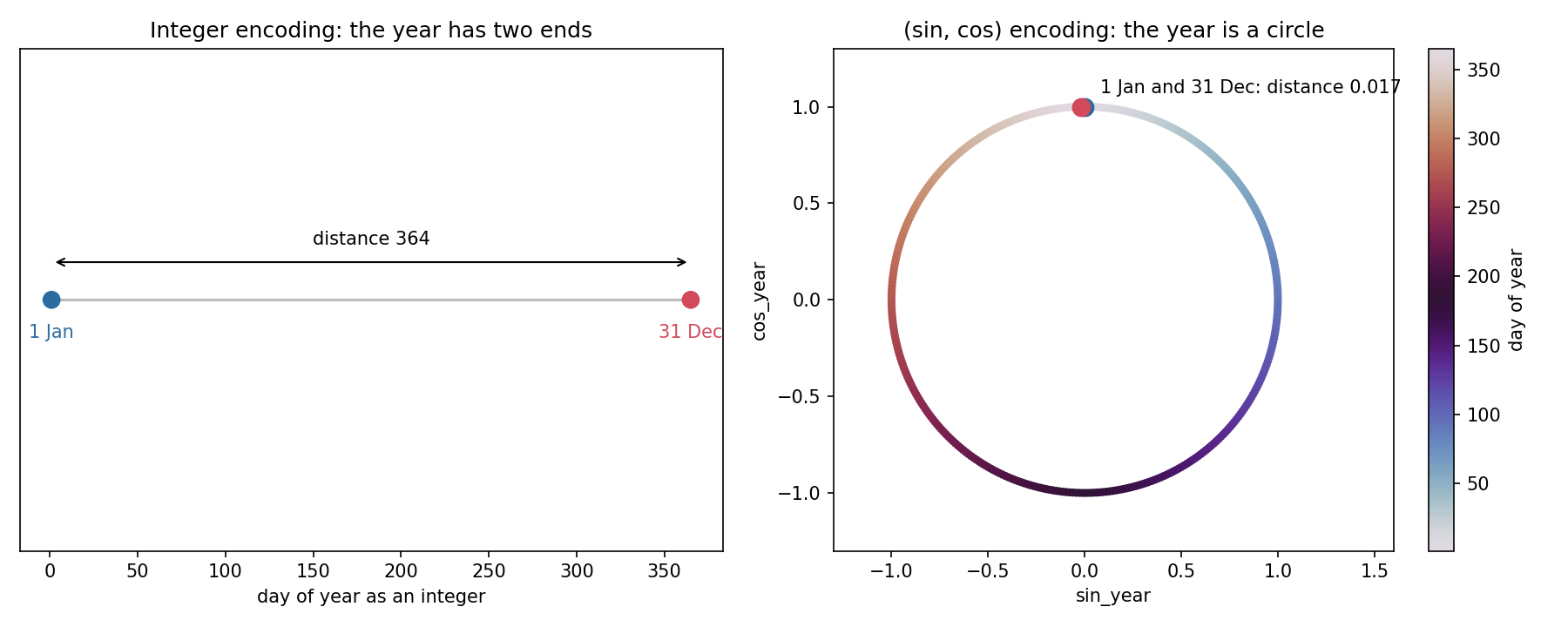
Q4. Cyclic time (B). As an integer, 31 December (365) and 1 January (1) are 364 apart, the maximum possible distance, although they are adjacent days with the same weather. Mapping the day $d$ to an angle puts the year on a circle:

\theta = \frac{2\pi (d-1)}{365}, \qquad (\text{sin\_year}, \text{cos\_year}) = (\sin\theta, \cos\theta).

Now consecutive days are always at the same distance (0.017), including across New Year. Two features are needed, because $\sin$ alone gives the same value to two different days (for instance early April and early September).

Left: on the integer line, 1 January and 31 December sit at opposite ends, 364 apart. Right: with sine and cosine features, the days form a circle and the two dates are neighbours, distance 0.017.

Q5. Soil moisture as a proxy (B). Soil moisture rises almost immediately when rain falls, so it records the physical footprint of a rain event: a strong proxy for "it has rained". It does not cause rain (A is backwards), and the other options are irrelevant. A caution worth knowing: precisely because it reacts to the rain you want to predict, soil moisture measured at or after the target time is leakage; only past values are fair features for forecasting.

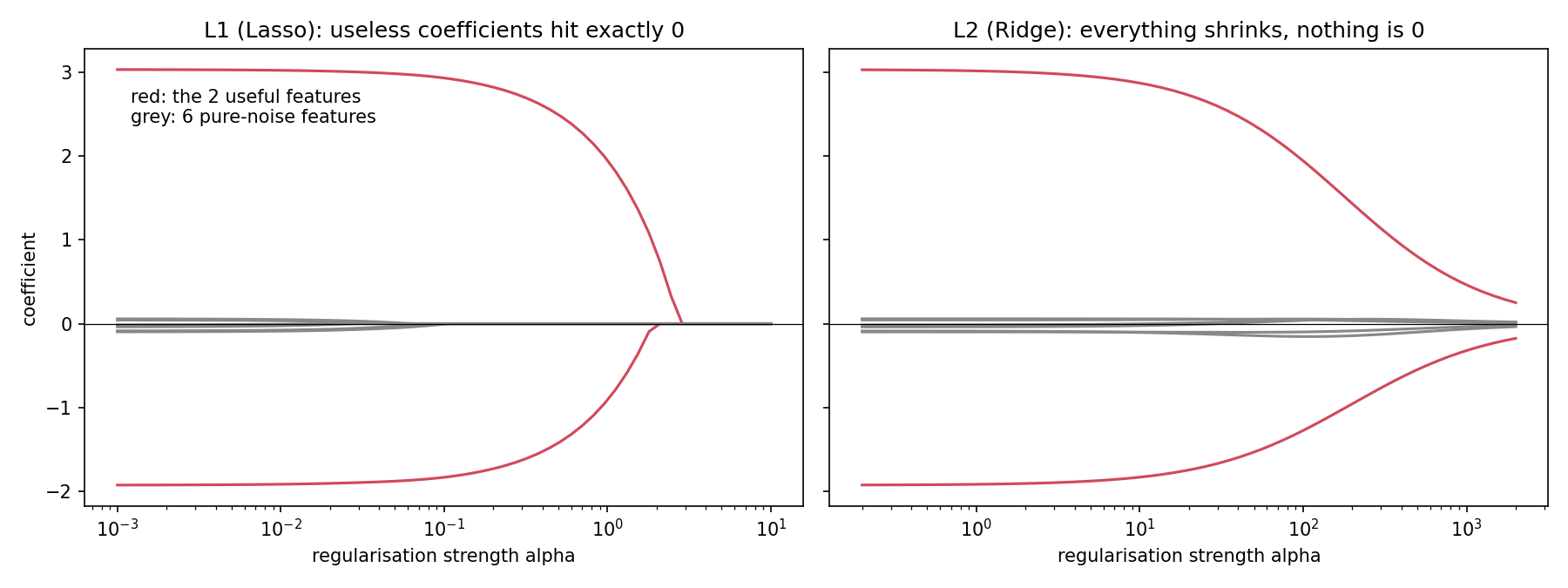
Q6. L1 versus L2 (A). L1 adds $\lambda\sum_j |w_j|$ to the loss, L2 adds $\lambda\sum_j w_j^2$ . The derivative of $\lambda|w|$ has constant size $\lambda$ however small $w$ is, so it can push a weak coefficient all the way to exactly 0; the derivative of $\lambda w^2$ , $2\lambda w$ , vanishes as $w \to 0$ , so L2 only shrinks. In our check with 2 useful and 6 noise features, Lasso returns exactly $0$ for all 6 noise coefficients, Ridge returns small non-zero values. L2 is used for regression too (B), and neither statement C nor D is true in general.

Coefficient paths as regularisation grows. With L1 the six noise coefficients become exactly zero early and stay there; with L2 all coefficients shrink smoothly but none reaches zero.

Q7. Elbow method (B). Plot the within-cluster sum of squares against $K$ . It always decreases as $K$ grows (more centroids, smaller clusters), so the minimum is useless; instead you look for the "elbow" where adding a cluster stops buying much. It has nothing to do with learning rates, t-SNE or outliers.

Part 2: Neural networks and deep learning

Q8. Backpropagation (B). It is the chain rule applied layer by layer: $\frac{\partial L}{\partial w^{(1)}} = \frac{\partial L}{\partial a^{(n)}}\frac{\partial a^{(n)}}{\partial a^{(n-1)}}\cdots\frac{\partial a^{(1)}}{\partial w^{(1)}}$ , computed from the output backwards so each factor is reused.

Q9. ReLU versus sigmoid (B). The sigmoid's derivative $\sigma'(z) = \sigma(z)(1-\sigma(z))$ is at most $1/4$ . Backpropagating through 10 sigmoid layers multiplies the gradient by at most $4^{-10} \approx 10^{-6}$ : the early layers barely learn. ReLU has derivative exactly 1 on its active units, so the signal passes through. It is also cheaper, not more expensive (A), and its output is unbounded, not in $[0,1]$ (C).

Q10. Dropout (B). At each training step a random subset of units is zeroed, so no unit can rely on a specific partner being present; the network must spread information redundantly, which behaves like averaging many thinned sub-networks. A describes a learning-rate scheduler, C weight decay, D data augmentation.

Q11. Scaled dot-product attention (C). $\operatorname{Attention}(Q,K,V) = \operatorname{softmax}\!\left(QK^\top/\sqrt{d_k}\right)V$ : queries are compared with keys, and the resulting weights average the values. B lists convolution hyperparameters.

Q12. PEFT (B). Methods such as LoRA freeze the pretrained weights and train a small number of new parameters (often well under 1 %), which cuts memory and compute and lets one base model carry many cheap task adapters. It does not extend the context window, still needs labelled data, and is not specific to vision.

Part 3: Computer vision and NLP

Q13. Pooling (B). Max pooling keeps the maximum of each small window (e.g. $2\times 2$ with stride 2), halving the height and width: fewer activations and less computation downstream, plus a little tolerance to small shifts. Pooling itself has no parameters; it reduces the parameters of later fully connected layers. Detecting edges (D) is the job of convolution kernels.

Q14. Real-time detection (C). YOLO predicts all boxes and classes in a single forward pass over the image, hence "You Only Look Once". ResNet is a classifier backbone, BERT a language model, U-Net a segmentation network.

Q15. Outlining a tropical depression (B). Outlining the exact area is semantic segmentation, a label per pixel, and U-Net (encoder-decoder with skip connections that keep fine spatial detail) is the classic architecture for it. VGG-16 classifies whole images; kNN and logistic regression are not image models.

Q16. Self-attention (A). Every token attends to every other token in the sequence, so its new representation mixes in context from the whole sentence ("bank" next to "river" versus next to "loan").

Q17. BERT pretraining (A). The original BERT was pretrained on two objectives: masked language modelling and Next Sentence Prediction. (Later work such as RoBERTa showed NSP is not essential, but it is part of the original model.) RLHF belongs to chat-tuned generative LLMs.

Part 4: Data science and evaluation

Q18. MAE versus RMSE for rainfall (B).

\text{MAE} = \frac{1}{n}\sum_i |e_i|, \qquad \text{RMSE} = \sqrt{\frac{1}{n}\sum_i e_i^2}.

Squaring makes large errors dominate. In our check, 100 errors of 2 mm give MAE = RMSE = 2; replacing one of them by a 120 mm storm miss moves MAE to 3.2 but RMSE to 12.2. Choose MAE when you do not want a few extreme storms to drive the metric (and choose RMSE when missing those storms is precisely what you must avoid). Note that C is false as stated: MAE is never higher than RMSE, but they can be equal.

Q19. Training MAE 0.02, validation MAE 0.25 (B). A large gap between excellent training error and much worse validation error is the signature of overfitting. Underfitting would show poor error on both.

Q20. RobustScaler (B). StandardScaler uses the mean and standard deviation, which a single extreme value distorts; RobustScaler uses $(x - \text{median})/\text{IQR}$ . In our check, one 999 % humidity reading inflates the standard deviation so much that all normal readings are squashed into a tiny interval around 0, while RobustScaler keeps them spread out normally. It does not map to $[0,1]$ (that is MinMaxScaler) and does not handle NaN for you.

Q21. Adam (B). Adam keeps an exponential average of past gradients (momentum) and of past squared gradients (the RMSProp idea), and divides one by the square root of the other, giving each parameter its own adaptive step size.

Q22. Missing values per column (B). df.isnull() gives a boolean table, and .sum() counts the True values column by column. describe() only shows the non-missing counts, indirectly; dropna() removes rows.

What to remember

Values that are physically impossible (999 % humidity) are missing data in disguise: convert them to NaN before computing any statistic.
Encode cyclic quantities (day of year, hour, wind direction) with a sine and a cosine, never a raw integer.
L1 gives exact zeros (feature selection), L2 gives smooth shrinkage; the reason is the slope of the penalty near 0.
RMSE and StandardScaler are sensitive to outliers, MAE and RobustScaler much less: pick according to whether extremes matter.
A good proxy feature can also be a leak: check that it is available before the moment you predict.

"""IOAI Philippines 2026 semi-finals theory: small numerical checks behind several answers,
and the figures of the correction."""
import numpy as np, pandas as pd, matplotlib
matplotlib.use("Agg"); import matplotlib.pyplot as plt
from sklearn.linear_model import Lasso, Ridge
from sklearn.preprocessing import StandardScaler, RobustScaler
rng = np.random.default_rng(0)

# Q4: day 365 and day 1 are 364 apart as integers but neighbours on the circle
def enc(d): a = 2 * np.pi * (d - 1) / 365; return np.array([np.sin(a), np.cos(a)])
print("Q4 integer gap:", 365 - 1, " circle gap:", round(np.linalg.norm(enc(365) - enc(1)), 4),
      " (vs days 182/183:", round(np.linalg.norm(enc(183) - enc(182)), 4), ")")

# Q6: Lasso sets useless coefficients exactly to 0, Ridge only shrinks them
X = rng.normal(size=(200, 8)); y = X[:, 0] * 3 - 2 * X[:, 1] + rng.normal(size=200)
print("Q6 Lasso:", np.round(Lasso(alpha=0.2).fit(X, y).coef_, 3))
print("Q6 Ridge:", np.round(Ridge(alpha=50).fit(X, y).coef_, 3))

# Q9: derivative of the sigmoid is at most 1/4, so 10 layers multiply gradients by <= 4^-10
print("Q9 max sigmoid gradient over 10 layers:", 0.25 ** 10, " ReLU (active units):", 1.0)

# Q18 / Q20: one extreme storm moves RMSE, StandardScaler far more than MAE, RobustScaler
err = np.full(100, 2.0); err_storm = err.copy(); err_storm[0] = 120
for name, e in [("no storm", err), ("one storm", err_storm)]:
    print(f"Q18 {name}: MAE={np.abs(e).mean():.2f}  RMSE={np.sqrt((e**2).mean()):.2f}")
h = np.r_[rng.normal(75, 8, 99), 999.0].reshape(-1, 1)   # humidity with one 999 % reading
print("Q20 StandardScaler: typical value scaled to",
      np.round(StandardScaler().fit_transform(h)[:3, 0], 3), " RobustScaler:",
      np.round(RobustScaler().fit_transform(h)[:3, 0], 3))

# Q22
df = pd.DataFrame({"temp": [30, None, 29], "humidity": [80, 999, None]})
print("Q22 df.isnull().sum():", df.isnull().sum().to_dict())

# Figure 1: cyclic encoding of the day of the year
d = np.arange(1, 366); a = 2 * np.pi * (d - 1) / 365
fig, ax = plt.subplots(1, 2, figsize=(12, 4.8))
ax[0].plot(d, np.zeros_like(d), "-", color="#bbb"); ax[0].scatter([1, 365], [0, 0], c=["#2b6ca3", "#d1495b"], s=80, zorder=3)
ax[0].annotate("", xy=(365, 0.15), xytext=(1, 0.15), arrowprops=dict(arrowstyle="<->"))
ax[0].text(183, 0.22, "distance 364", ha="center"); ax[0].set_ylim(-1, 1); ax[0].set_yticks([])
ax[0].text(1, -0.15, "1 Jan", ha="center", color="#2b6ca3"); ax[0].text(365, -0.15, "31 Dec", ha="center", color="#d1495b")
ax[0].set_xlabel("day of year as an integer"); ax[0].set_title("Integer encoding: the year has two ends")
sc = ax[1].scatter(np.sin(a), np.cos(a), c=d, cmap="twilight", s=12)
ax[1].scatter(*enc(1), c="#2b6ca3", s=90, zorder=3); ax[1].scatter(*enc(365), c="#d1495b", s=90, zorder=3)
ax[1].text(0.08, 1.07, "1 Jan and 31 Dec: distance 0.017", fontsize=10)
ax[1].set_aspect("equal"); ax[1].set_xlabel("sin_year"); ax[1].set_ylabel("cos_year"); ax[1].set_xlim(-1.3, 1.6); ax[1].set_ylim(-1.3, 1.3)
ax[1].set_title("(sin, cos) encoding: the year is a circle"); fig.colorbar(sc, ax=ax[1], label="day of year")
fig.tight_layout(); fig.savefig("figures/cyclic.png", dpi=150, facecolor="white")

# Figure 2: L1 versus L2 coefficient paths
alphas = np.logspace(-3, 1, 60)
L = np.array([Lasso(alpha=al).fit(X, y).coef_ for al in alphas])
R = np.array([Ridge(alpha=al * 200).fit(X, y).coef_ for al in alphas])
fig, ax = plt.subplots(1, 2, figsize=(12, 4.5), sharey=True)
for k in range(8):
    col = "#d1495b" if k < 2 else "#888"
    ax[0].semilogx(alphas, L[:, k], color=col); ax[1].semilogx(alphas * 200, R[:, k], color=col)
ax[0].set_title("L1 (Lasso): useless coefficients hit exactly 0"); ax[1].set_title("L2 (Ridge): everything shrinks, nothing is 0")
ax[0].set_xlabel("regularisation strength alpha"); ax[1].set_xlabel("regularisation strength alpha"); ax[0].set_ylabel("coefficient")
for a_ in ax: a_.axhline(0, color="k", lw=0.6)
ax[0].text(0.0012, 2.4, "red: the 2 useful features\ngrey: 6 pure-noise features", fontsize=10)
fig.tight_layout(); fig.savefig("figures/l1_l2.png", dpi=150, facecolor="white")

Theory Assessment