Theory & Technical Concepts

The problem in brief

This is a one-hour paper of 30 single-answer multiple-choice questions, from the Philippine national finals for IOAI 2026. It has three sections of ten questions: mathematics and classical machine learning, deep-learning mechanics, and generative AI and safety. The organisers published only the questions (in the ioaiph/2026 GitHub repository), not the answers. Every answer below is derived here, and each numeric one is checked in solution.py. In the published PDF a few mathematical symbols failed to render (the $K$ in question 9, option D of question 14, the $F(x)$ in question 17, the $q(x_t\mid x_0)$, $T\to\infty$ and $\mathcal N(0,I)$ in question 26). We read them in the obvious way.

How you are scored

One point per correct answer, out of 30. No pass mark is published.

The full solution

Section 1: Mathematics and classical ML

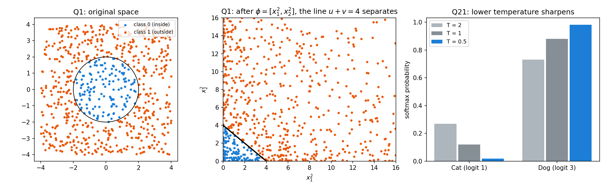
1. B, $\phi=[x_1^2,x_2^2]$. The class boundary is $x_1^2+x_2^2=4$. In the coordinates $u=x_1^2,\ v=x_2^2$ it becomes the straight line $u+v=4$. The other maps only add linear or odd functions, which cannot tell a point from its mirror image across the origin. Fitting a linear classifier confirms it: 100 % training accuracy with B, 80 % (the majority class) with A, C and D.

2. C, a saddle point. At a critical point, positive Hessian eigenvalues mean the surface curves up in that direction, and negative ones mean it curves down. $\lambda_1=5>0$ and $\lambda_2=-3<0$: up one way and down the other, so a saddle. Think of $f=2.5x^2-1.5y^2$.

3. B, the diamond. The L1 constraint region $\lvert w_1\rvert+\lvert w_2\rvert\le t$ has corners on the axes. The elliptical loss contours usually first touch it at a corner, where one coordinate is exactly 0. The L2 ball is round, so the contact point is generically off the axes.

4. B, biased low. For the MLE, $\mu$ is replaced by the sample mean $\bar x$, and

$$\mathbb E\Big[\tfrac1N\textstyle\sum(x_i-\bar x)^2\Big] = \tfrac{N-1}{N}\,\sigma^2 < \sigma^2 .$$

With $N=5$, a simulation gives 0.80 for a true variance of 1. This is why the unbiased estimator divides by $N-1$. If $\mu$ were the true mean, the formula would be unbiased. That reading is not the MLE, so B is the intended answer.

5. B, boundary 4, margin 4. The hard-margin SVM puts the boundary halfway between the support vectors, at $x=4$. The constraints $6w+b=1$ and $2w+b=-1$ give $w=\tfrac12$, so the margin width is $2/\lvert w\rvert=4$, the distance between the two support vectors. Option A (margin 2) uses the other convention, the distance from the boundary to one support vector, so the question is slightly ambiguous. With the standard $2/\lVert w\rVert$ definition, the answer is B.

6. B. Almost all the variance (50 against 0.001) lies along one direction: the points lie on a line, and projecting onto the first principal component loses about 0.002 % of the variance. Option D is wrong because principal components are mixtures of $x_1$ and $x_2$, not the original features.

7. A, 2.4. $L'(w)=2w=6$, so $w\leftarrow 3-0.1\cdot6=2.4$.

8. B. "Naive" refers to the assumption $P(x_1,\dots,x_d\mid y)=\prod_j P(x_j\mid y)$: features are conditionally independent given the class.

9. B, the inertia. Each K-means step can only lower the within-cluster sum of squares, or leave it unchanged. The assignment step gives every point its nearest centroid, and the update step moves each centroid to the mean of its points, which minimises the squared distances for that cluster. The silhouette score, the distances between centroids and agreement with true labels can all move either way.

10. C. The parent node has entropy 1 bit. The information gains are: A 0.531, B 0, C 1.0 (two pure children), D 0.029.

Section 2: Deep-learning mechanics

11. B, the weights stay exactly zero. Zero weights make the hidden pre-activations 0, so $h=\mathrm{ReLU}(0)=0$. The output-layer weight gradient is $\delta\,h^\top=0$, and the gradient flowing back to the hidden layer is $W_2^\top\delta=0$, because $W_2=0$. The only nonzero gradient is on the output bias, which solution.py confirms in PyTorch. That makes D half true: one bias updates, not "the biases". Since $h$ stays 0, nothing else will ever move: the network is dead. Option C, where all neurons learn the same feature, is what happens with a constant nonzero initialisation. That is the classic symmetry problem, but it is not this setup.

12. A, $28\times28\times10$. The spatial size is $(32-5+0)/1+1=28$, and there is one output channel per filter.

13. B, $1\times1\times256\times64$. Each filter spans all 256 input channels, so there are $256\cdot64=16\,384$ weights. D is the same number written without the $1\times1$ factor. B is the form that shows where it comes from.

14. B, $5\times5$. Each $3\times3$ layer adds 2 to the receptive field: $1+2+2=5$. That is why two stacked $3\times3$ convolutions replace one $5\times5$ with fewer parameters ($18$ against $25$ per channel pair).

15. B. $\sigma'(z)=\sigma(z)(1-\sigma(z))\le 0.25$, with the maximum at $z=0$. Backpropagation through $L$ sigmoid layers multiplies $L$ such factors, at most $0.25^L$, so gradients vanish. ReLU has derivative exactly 1 on active units. (Strictly, the bound is $\le 0.25$, not $<0.25$.)

16. B. At inference, BatchNorm uses the running mean and variance accumulated during training, so a prediction does not depend on the other examples in the batch.

17. B. With $y=F(x)+x$, $\dfrac{\partial y}{\partial x}=\dfrac{\partial F}{\partial x}+I$. The identity term carries the gradient straight to earlier layers, even when $\partial F/\partial x$ is small.

18. B, 4 times. The attention matrix is $N\times N$, and $(1024/512)^2=4$.

19. C, do nothing (in the standard implementation). Modern frameworks use inverted dropout: during training, the kept activations are divided by $1-p$, so their expected value is already correct, and at inference the layer is the identity. solution.py checks this on PyTorch's Dropout. Option A, multiplying the weights by $1-p=0.5$ at test time, is the original 2014 formulation, which gives the same expected value. Since the question says "standard implementation", C is the better answer, but expect some graders to want A.

20. B. Taking the maximum over a small window gives an output that barely changes when the input shifts by a pixel or two. Max pooling gives no invariance to rotation, colour or scale.

Section 3: Generative AI and safety

21. B. Dividing the logits by $T=0.5$ doubles the gap between them. Softmax goes from $(0.119,\,0.881)$ to $(0.018,\,0.982)$: the distribution sharpens and the order never changes.

22. A. Self-attention treats its input as a set: permuting the tokens just permutes the outputs (strictly, it is permutation equivariant). Without positional information, the model cannot tell "the dog bit the man" from "the man bit the dog".

23. B. Following instructions is taught by supervised fine-tuning on instruction-response pairs. RLHF usually comes after SFT and aligns the model with preferences.

24. B. This is Goodhart's law: once the learned reward becomes the target, the policy exploits its errors. That is why RLHF adds a KL penalty towards the reference model.

25. B. FGSM computes $x' = x+\epsilon\,\mathrm{sign}(\nabla_x L)$, a step in input space that increases the loss. The weights stay fixed.

26. B. The forward process repeatedly shrinks the signal and adds Gaussian noise: $x_t=\sqrt{\bar\alpha_t}\,x_0+\sqrt{1-\bar\alpha_t}\,\varepsilon$ with $\bar\alpha_t\to0$. In the limit it becomes $\mathcal N(0,I)$, which is why generation can start from pure noise.

27. B. BPE repeatedly merges the most frequent adjacent pair of symbols in the training corpus.

28. B. The retrieved passages are inserted into the prompt as context. The model's weights do not change.

29. B. Equalized odds asks for equal true-positive rates (and equal false-positive rates) across groups. "80 % of qualified men and of qualified women" is a statement about TPR. Metric A, equal overall approval rates, is demographic parity. Strictly, Metric B shows only the TPR half of equalized odds (that half alone is called equal opportunity), but it is the one that matches.

30. B. An RNN's hidden state $h_t$ depends on $h_{t-1}$, so training must step through time in order. A Transformer computes all positions at once with matrix products, which suits GPUs.

Results

#	answer	#	answer	#	answer
1	B	11	B	21	B
2	C	12	A	22	A
3	B	13	B	23	B
4	B	14	B	24	B
5	B	15	B	25	B
6	B	16	B	26	B
7	A	17	B	27	B
8	B	18	B	28	B
9	B	19	C	29	B
10	C	20	B	30	B

Four questions depend on a convention, flagged above: 5 (what "margin" means), 11 (B against the half-true D), 13 (B and D are the same number) and 19 (inverted dropout C against the original A).

What to remember

• Check numeric options by computing them. Information gain, convolution shapes, receptive fields and a gradient step each take one line, and a quick PyTorch check settles initialisation and dropout questions without arguing.
• A feature map can turn a curved boundary into a straight one ($x_1^2+x_2^2=4$ becomes $u+v=4$). This is the intuition behind kernels.
• Know the two conventions behind common traps: SVM margin (full width $2/\lVert w\rVert$ or half of it) and dropout (inverted, or rescaled at test time).
• Zero initialisation is worse than symmetric. With ReLU and zero weights the network gets no weight gradient at all. With a constant nonzero initialisation, the neurons stay identical.
• The fairness criteria have short definitions. Demographic parity means equal approval rates. Equalized odds means equal TPR and FPR. Equal opportunity means equal TPR only.