The problem in brief
You must count the people in photographs of busy streets and shopping areas (1024 × 768 pixels). The 100 training images come with a point on every head; the 216 test images come with nothing. The deliverable is one number per test image. Pretrained models are explicitly allowed (the rules name YOLOv8 and CSRNet as examples).
The data comes from the Kaggle competition archive. The test counts are private and we never submitted anything, so all scores below are 5-fold cross-validation on the 100 labelled images.
How you are scored
Root mean squared error between predicted and true counts:
Lower is better. Because the errors are squared, a few large mistakes on very crowded images dominate the score.
What to aim for. The only entry on the public leaderboard is the organisers' baseline, at 143.9. No other threshold is published.
First look at the data
Counts range from 15 to 539 people (median 90, mean 126, standard deviation 105). Simply predicting the training mean for every image gives an RMSE of 105.5 in cross-validation, already better than the published baseline. People near the camera are large; people at the back are a few pixels wide and overlap each other, which is why the hints warn that a person detector struggles with dense crowds: it cannot draw a box around a head it cannot separate from its neighbours.
A first baseline
| approach | CV RMSE |
|---|---|
| organisers' baseline (public leaderboard, different images) | 143.9 |
| predict the training mean | 105.5 |
The key idea
Do not detect people: estimate a density and integrate it. Put a small Gaussian blob of total mass 1 on every annotated head. The resulting density map is zero where there is nobody, high where heads are packed, and its integral is exactly the number of people:
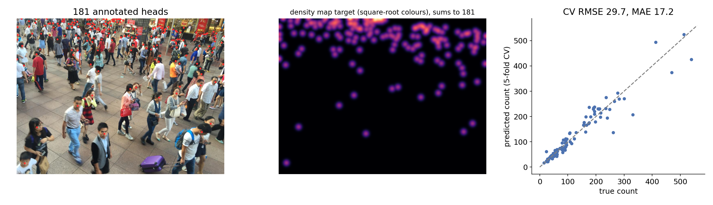
A fully convolutional network is trained to reproduce pixel by pixel, and the predicted count is the sum of the predicted map. This changes the problem in three good ways:
- No need to separate people. Two overlapping heads simply add up to a mass of 2. The network only has to recognise "head-like texture at this scale", which is local and works the same for one person or a thousand.
- Much more supervision. A count is one number per image; a density map gives a target for every location, so 100 images become tens of thousands of supervised patches.
- Crops are allowed. Since a count is additive, any crop of an image has a known count (the sum of the density inside it). We train on random 256 × 256 crops, which is both data augmentation and a way to fit in memory.
The architecture is CSRNet: the first ten convolutional layers of an ImageNet-pretrained VGG16 (stride 8, they already know edges, textures and object parts), followed by six dilated 3 × 3 convolutions. Dilation spaces the taps of each filter apart, so the receptive field grows to cover a whole crowd region without further pooling, and the output keeps a resolution of 1/8 of the input.
The full solution
- Resize images to half resolution (512 × 384) and build density maps with pixels, renormalised so that blobs cut by the border still sum to the exact count; downsample them by 8 with a sum (not a mean), multiplied by 100 so that the targets are not tiny numbers.
- CSRNet with VGG16-BN weights (
timm/vgg16_bn.tv_in1k, safetensors), the first two VGG blocks frozen to save memory and to keep generic low-level filters. - Train 100 epochs on random 256 × 256 crops with horizontal flips, batch 4, pixel-wise squared error on the density, Adam with learning rate and cosine decay (about 5 minutes on the Apple GPU).
- Predict on the whole half-resolution image and sum the map:
def count(m, X):
    return [float(m(to_tensor(x)).sum()) / 100 for x in X]   # integral of the density = number of people
- For the submission, train on all 100 images and predict the 216 test images.
Results
5-fold cross-validation on the 100 labelled images (official test counts private).
| approach | RMSE | MAE |
|---|---|---|
| predict the training mean | 105.5 | |
| CSRNet, half resolution, fold 0 only | 34.4 | 19.5 |
| CSRNet, 0.75 resolution, fold 0 only (failed) | 48.6 | 29.2 |
| CSRNet, half resolution, 5-fold CV (final) | 29.7 | 17.2 |
The final model reaches an RMSE of 29.7 and a mean absolute error of 17 people, against 105.5 for the constant prediction and 143.9 for the published baseline. The folds vary a lot (RMSE 16.8 to 34.8), and the right panel above shows why: almost all of the squared error comes from a handful of very dense images (261 people predicted as 136, 539 as 426). Without the five worst images the RMSE would be 17.4. Training at 0.75 resolution with the same crop size was worse on fold 0: each crop then covers less of the scene, and with only 80 training images context seems to matter more than detail.
What to remember
- Counting is integration. Turning points into a density map makes counting a dense regression problem that handles occlusion naturally and gives far more supervision than one number per image.
- Additive targets allow crops. When the label of a part is known (here, the mass inside the crop), random crops are free augmentation and save memory.
- Pretrained convolutional features transfer to new tasks. Ten VGG layers trained on ImageNet plus a small new head learn a good density estimator from just 100 images.
- Dilated convolutions enlarge the receptive field without losing resolution, which is what dense prediction needs.
- RMSE is ruled by the worst cases. Look at the largest errors first: here a few very crowded images account for most of the score.
Note on the code. The full
solution.pybelow reproduces the setup that produced the reported score, but it was not re-run end to end after it was assembled.