IOAI Perú: Information Retrieval Challenge

The problem in brief

You are given 97 Spanish Wikipedia-style articles about Peru (history, food, geography, politics, music...) and natural-language questions such as "¿Qué ingredientes lleva el ceviche peruano tradicional?". For each question, your search engine must rank the articles from most to least relevant. The organisers provide a working TF-IDF baseline in a notebook and ask for at least one stronger model (BM25, embeddings, anything), an evaluation with standard IR metrics on 30 development questions that come with relevance judgments, and a ranked list for 20 test questions. The final deliverable also includes pushing the model to the Hugging Face Hub, which we skip: it needs an account and adds nothing to the method.

How you are scored

For each query the system returns a ranked list. With $\mathcal{R}_q$ the set of documents judged relevant for query $q$ and $\text{rel}(k) = 1$ if the document at rank $k$ is relevant:

$$P@10 = \frac{1}{10}\sum_{k=1}^{10}\text{rel}(k), \qquad R@10 = \frac{1}{|\mathcal{R}_q|}\sum_{k=1}^{10}\text{rel}(k),$$ $$AP(q) = \frac{1}{|\mathcal{R}_q|}\sum_{k=1}^{10} \text{rel}(k)\, P@k, \qquad \text{MAP} = \frac{1}{|Q|}\sum_{q} AP(q).$$

AP rewards putting the relevant documents early: a hit at rank 1 contributes $1/|\mathcal{R}_q|$, a hit at rank 10 behind 9 misses only $0.1/|\mathcal{R}_q|$. The official notebook computes AP on the top-10 list, and so do we. MAP is the main number. The test judgments are private and no threshold is published, so all scores below are on the 30 development queries, and "beating the official TF-IDF baseline" (MAP 0.326) is the natural target.

First look at the data

Before building anything, read the relevance judgments. They are surprising:

• Each query has between 2 and 10 relevant documents, and the lists are always sorted by document number and capped at 10. They look machine-generated rather than written by a careful annotator.
• The judgments are noisy. For "¿Quién fue José de San Martín y qué hizo en Perú?" the article José de San Martín is not judged relevant, while Pisco del Perú and Geografía del Perú are. For "¿Cuál es el origen del Imperio Incaico?", the article Imperio incaico is missing too.
• A handful of broad overview articles appear everywhere: Historia del Perú is relevant to 18 of the 30 queries, Literatura del Perú to 15.

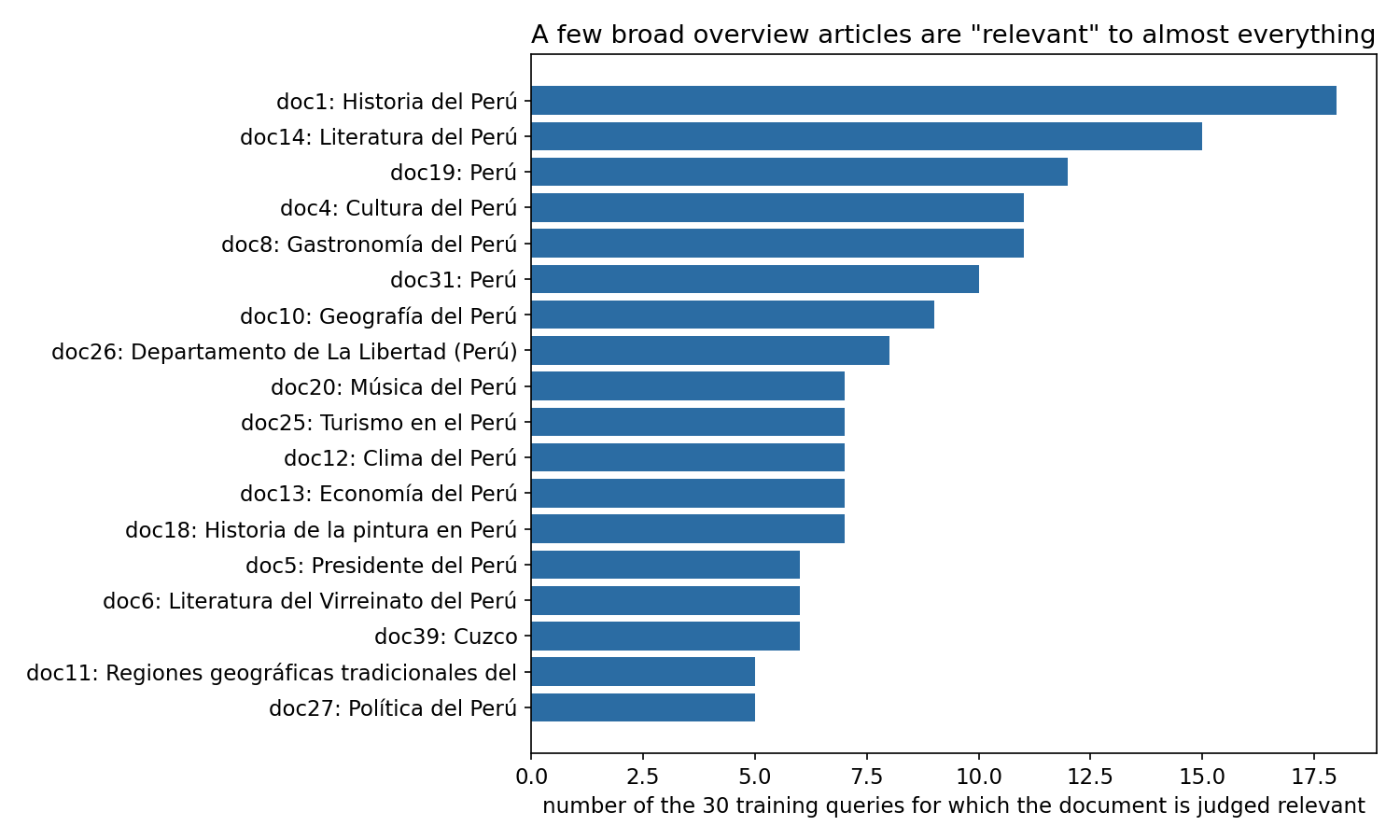
This changes the game. Any method is measured against these labels, so a "smarter" retriever that returns José de San Martín first for the San Martín question is actually penalised. Scores will be low for every method (a MAP around 0.3 to 0.4), and differences of 0.02 between methods on 30 queries are within noise.

A first baseline

The notebook's baseline: normalise Spanish text (lowercase, remove punctuation and digits, remove stopwords, Snowball stemming so that peruanos, peruana and peruano all become peruan), build TF-IDF vectors and rank by cosine similarity. We reproduce its numbers exactly: MAP 0.326, P@10 0.400.

The classic upgrade is BM25, which saturates term frequency (the 10th occurrence of "inca" adds much less than the first) and normalises by document length:

$$\text{BM25}(q, d) = \sum_{t \in q} \text{idf}(t)\,\frac{f_{t,d}\,(k_1+1)}{f_{t,d} + k_1\left(1 - b + b\,\frac{|d|}{\overline{|d|}}\right)} .$$

On this data it gives MAP 0.327, no better: we tried 16 combinations of $k_1 \in \{0.9, 1.2, 1.5, 2\}$ and $b \in \{0.3, 0.5, 0.75, 0.9\}$ and all land between 0.318 and 0.337. A dense retriever (multilingual-e5-small sentence embeddings) is worse still, 0.283, precisely because it is good at semantic matching: it finds the specific article, which the judgments often do not reward.

The key idea

Two ideas, one standard and one specific to this dataset.

1. Fuse scorers that make different mistakes. TF-IDF, BM25 and embeddings look at the text differently: exact stemmed words, saturated word counts, and meaning (synonyms, paraphrases, "comida" versus "gastronomía"). Their raw scores live on different scales (cosine in $[0, 1]$, BM25 up to 30), so we standardise each one per query before averaging:

$$z_m(q,d) = \frac{s_m(q,d) - \mu_m(q)}{\sigma_m(q)}, \qquad s_{\text{hybrid}}(q, d) = \tfrac{1}{3}\left(z_{\text{tfidf}} + z_{\text{bm25}} + z_{\text{dense}}\right).$$

A document that all three scorers like rises; a document that only one scorer likes by accident is diluted. This lifts MAP to 0.346, the first method that beats the baseline, even though the dense model alone was the worst.

2. Learn a document prior from the training judgments. The figure above says that, in this collection as judged, some documents are relevant far more often than others. In probabilistic IR terms, the probability of relevance factorises into a query-dependent part and a query-independent part, the prior $P(\text{rel} \mid d)$, which classical web search estimates from PageRank or click counts. Here the 30 training queries give a direct estimate: the number of queries $n_d$ for which $d$ was relevant. We add it, standardised, to the hybrid score:

$$s(q, d) = s_{\text{hybrid}}(q,d) + \alpha\, z\big(\log(1 + n_d)\big), \qquad \alpha = 0.5 .$$

The logarithm stops Historia del Perú from dominating every ranking; the query-dependent part still decides among the rest.

To measure this honestly we use leave-one-query-out: when scoring query $q$, $n_d$ is counted on the other 29 queries only. Otherwise the prior would literally contain the answer. Even so, MAP jumps to 0.408. Be clear about what this means: the prior does not make the engine understand Peru better, it learns how the annotators labelled. It is legitimate (it uses training data only, never the test judgments) and it is exactly what a learning-to-rank system does with a "document popularity" feature, but it only helps on the test set if the test judgments were produced the same way, which the identical file format strongly suggests.

The full solution

1. Normalise title + text of each article with the official Spanish pipeline (keeps the baseline comparable).
2. TF-IDF + cosine and BM25 (rank_bm25, default $k_1=1.5$, $b=0.75$) on the stemmed tokens.
3. Dense scores. Articles average 1 600 words, more than the encoder's 512-token window, so we cut each one into overlapping 200-word passages (stride 150), embed them with intfloat/multilingual-e5-small (with its required query: / passage: prefixes) and score a document by the mean of its 3 best passages. Taking only the best passage (0.274) or the mean of all passages (0.227) was worse: a long article should get credit for a few strongly matching passages, not be diluted by the unrelated ones.

sim = enc.encode(["query: " + q for q in qs], normalize_embeddings=True) @ P.T
S_dense = np.stack([np.sort(sim[:, owner == j], axis=1)[:, -3:].mean(1)
                    for j in range(n_docs)], axis=1)

4. Fuse with per-query z-scores, then add the prior $\alpha\,z(\log(1+n_d))$ computed on all 30 training queries for the test predictions (leave-one-out for the evaluation).
5. Write the top 50 documents per test query in the official format query_id 0 doc_id rank score run_id.

Results

On the 30 development queries (official metric code; test judgments are private):

approach	P@10	R@10	MAP
TF-IDF + cosine (official baseline)	0.400	0.481	0.326
TF-IDF, sublinear tf + bigrams	0.367	0.449	0.326
BM25, best of 16 $(k_1, b)$ settings	0.367	0.448	0.337
dense e5-small, best passage	0.353	0.423	0.274
dense e5-small, mean of top-3 passages	0.350	0.420	0.283
TF-IDF + dense	0.383	0.460	0.321
TF-IDF + log document length	0.393	0.468	0.330
hybrid TF-IDF + BM25 + dense	0.403	0.484	0.346
hybrid + learned document prior (leave-one-query-out)	0.470	0.541	0.408

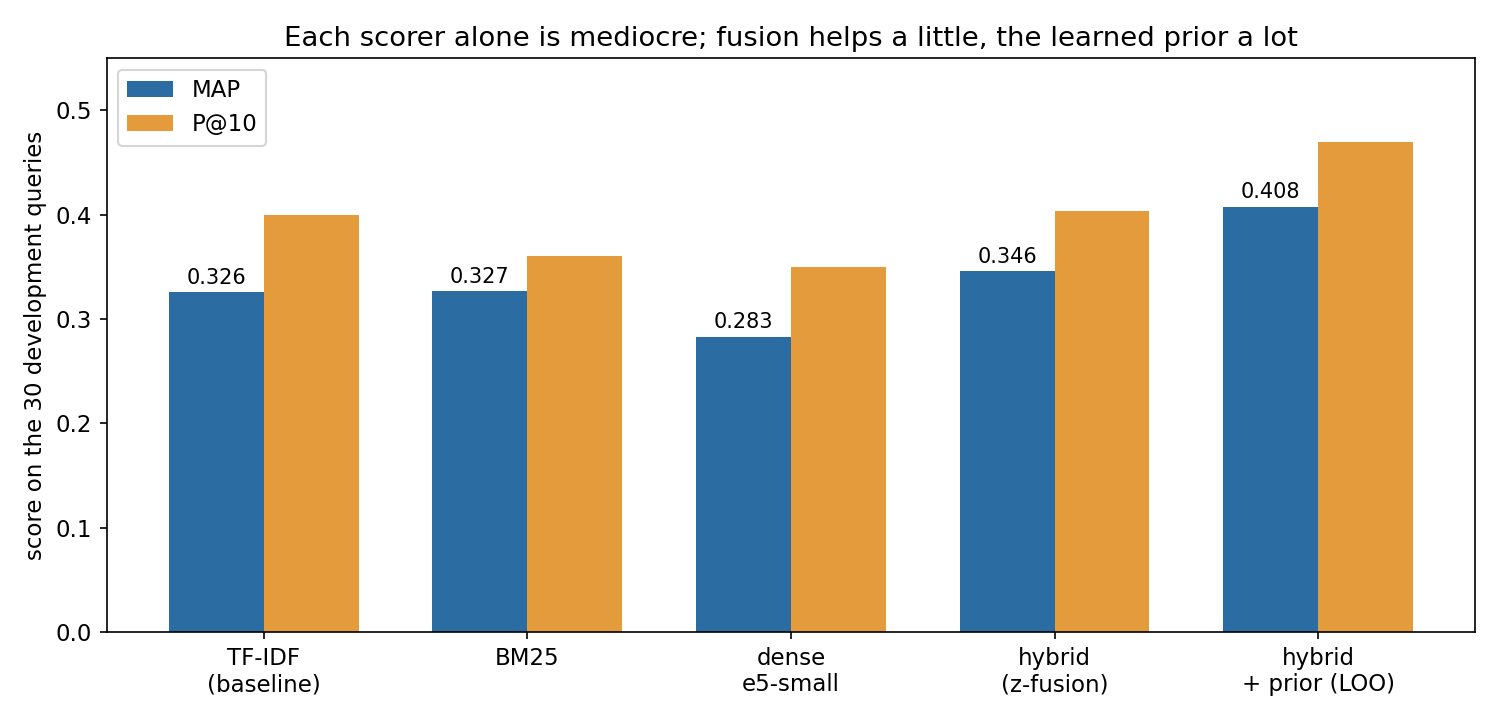
A word of caution on the table: with 30 queries, one query moving by 0.3 AP changes MAP by 0.01, and we compared about 25 configurations on the same queries. Only the prior's gain (+0.06 over the hybrid) is clearly larger than that noise; the ranking among the other rows should not be over-interpreted.

What to remember

• Read the labels before the data. The judgments define the task; here they reward broad overview articles, which explains why "smarter" semantic search scores lower.
• Fuse scorers on a common scale. Per-query z-scores (or reciprocal rank fusion) let lexical and dense retrievers vote together; the combination beats each one.
• Long documents need passages. Embed chunks and aggregate (top-k mean), instead of truncating at the model's window.
• A query-independent prior is a real feature, but estimate it leave-one-out, and say clearly that it learns the labelling process, not the language.
• Small evaluation sets are noisy. With 30 queries, treat differences of a couple of points as ties and prefer simple, principled choices over the best row of a big grid.