← Retour à l'épreuve

Kazakhstan FAIO 2025 · Correction IOAI Training

Problem 3: Medicine

Cette page donne toute la méthode. Lisez-la une fois que vous avez cherché.

Métrique
exact answer
Évaluée sur
written answers
Notre score
0.3333 = 1/3, checked 3 ways
Niveau attendu
the exact value to 4 decimals (10 points)

Niveau attendu atteint

Nous avons résolu l'épreuve nous-mêmes : téléchargé les données, mené les expériences et mesuré le score ci-dessous. L'énoncé et les données appartiennent à leurs organisateurs. Cette correction est rédigée en anglais.

The problem in brief

A disease affects 1 % of the population. A new test detects it in 99 % of sick people and correctly reports "negative" for 98 % of healthy people. Someone chosen at random tests positive: how likely is it that they are really sick? The answer is a probability written with four decimals. This is the textbook illustration of Bayes' theorem, and of the base-rate fallacy: most people, including many doctors in classic surveys, answer "about 99 %". The truth is very different.

How you are scored

A single exact answer with four decimals, worth 10 points. Our answer, obtained exactly with fractions and confirmed by a simulation of two million people:

0.3333\boxed{0.3333}

First look: name the numbers

Write SS for "sick" and ++ for "the test is positive". The statement gives three numbers, each with a standard name you will meet again in classifier evaluation:

quantityvaluename
P(S)P(S)0.010.01prevalence, the prior
P(+∣S)P(+ \mid S)0.990.99sensitivity, or recall / true positive rate
P(−∣Sˉ)P(- \mid \bar S)0.980.98specificity, so P(+∣Sˉ)=0.02P(+ \mid \bar S) = 0.02 is the false positive rate

The question asks for P(S∣+)P(S \mid +), the precision of the test (positive predictive value). The trap is to confuse P(S∣+)P(S \mid +) with P(+∣S)=0.99P(+ \mid S) = 0.99: they are conditional probabilities in opposite directions.

The key idea

Bayes' theorem flips the conditioning, and the law of total probability gives the denominator by splitting the positives into those who are sick and those who are not:

P(S∣+)=P(+∣S) P(S)P(+),P(S \mid +) = \frac{P(+ \mid S)\,P(S)}{P(+)}, P(+)=P(+∣S) P(S)+P(+∣Sˉ) P(Sˉ).P(+) = P(+ \mid S)\,P(S) + P(+ \mid \bar S)\,P(\bar S).

Plugging in the numbers:

P(+)=0.99×0.01+0.02×0.99=0.0099+0.0198=0.0297,P(+) = 0.99 \times 0.01 + 0.02 \times 0.99 = 0.0099 + 0.0198 = 0.0297, P(S∣+)=0.00990.0297=13≈0.3333.P(S \mid +) = \frac{0.0099}{0.0297} = \frac{1}{3} \approx 0.3333 .

Notice the neat structure: 0.01980.0198 is exactly twice 0.00990.0099, because the false positive rate (2%2\%) times the healthy share (99%99\%) is twice the prevalence (1%1\%) times the sensitivity (99%99\%). For every true positive there are two false positives, hence one chance in three.

The same thing with natural frequencies

Imagine 10 000 people.

  • 100 are sick; the test flags 0.99×100=990.99 \times 100 = 99 of them.
  • 9 900 are healthy; the test wrongly flags 0.02×9 900=1980.02 \times 9\,900 = 198 of them.

Among the 99+198=29799 + 198 = 297 positive results, only 99 belong to sick people: 99/297=1/399/297 = 1/3.

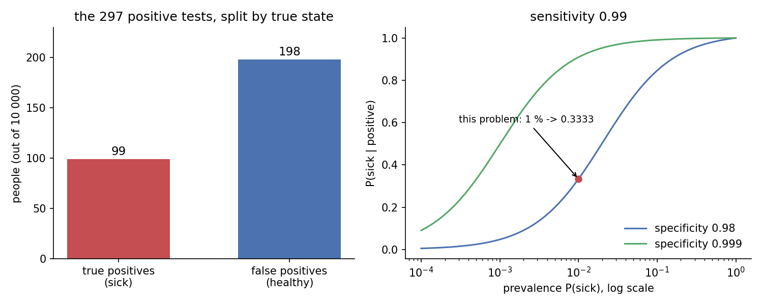
Left: among 10 000 people, the 297 positive tests split into 99 true positives and 198 false positives. Right: P(sick | positive) as a function of the prevalence on a log scale, for sensitivity 0.99 and specificity 0.98 (this problem, red dot at 1 % giving 0.3333) or 0.999 (a much better curve).

Why is the answer so low although the test is "99 % accurate"? Because the disease is rare. The healthy group is 99 times larger than the sick group, so even a small false positive rate applied to that huge group produces more false alarms than there are sick people to detect. The right panel shows how strongly the answer depends on the prior: the same test would give a posterior above 0.9 if 20 % of the people tested were sick, and a nearly useless 0.05 at prevalence 0.1 %.

What would actually help

  • Better specificity matters more than better sensitivity here: with 99.9 % specificity the posterior jumps to 0.0099/(0.0099+0.00099)≈0.9090.0099/(0.0099 + 0.00099) \approx 0.909.
  • A second, independent positive test uses 1/31/3 as the new prior: 0.99⋅1/30.99⋅1/3+0.02⋅2/3=99103≈0.9612\frac{0.99 \cdot 1/3}{0.99 \cdot 1/3 + 0.02 \cdot 2/3} = \frac{99}{103} \approx 0.9612. This is why screening positives are always confirmed by a second test.

The full solution

solution.py computes the answer three independent ways:

from fractions import Fraction as F
prev, sens, spec = F(1, 100), F(99, 100), F(98, 100)
p_pos = sens * prev + (1 - spec) * (1 - prev)   # 297/10000
post = sens * prev / p_pos                      # exactly 1/3
  • exact fractions with Bayes' formula: 1/31/3;
  • natural frequencies on 10 000 people: 99/297=1/399/297 = 1/3;
  • a Monte Carlo simulation of 2 000 000 random people: 0.33180.3318, within sampling noise of 0.33330.3333 (only about 59 000 of them test positive, so the standard error is about 0.0020.002).

Answer to submit, rounded to four decimals: 0.3333.

Results

approachvalueverdict
Bayes' theorem with exact fractions1/3=0.33331/3 = 0.3333correct
natural frequencies (10 000 people)99/297=0.333399/297 = 0.3333correct
Monte Carlo, 2 000 000 people0.3318agrees within noise
confusing P(S∣+)P(S \mid +) with the sensitivity P(+∣S)P(+ \mid S)0.9900wrong: base-rate fallacy
forgetting the false positives in the denominator1.0000wrong
using P(+∣Sˉ)=0.98P(+ \mid \bar S) = 0.98 instead of 0.020.020.0101wrong: specificity is about negatives

What to remember

  • P(A∣B)≠P(B∣A)P(A \mid B) \ne P(B \mid A). Bayes' theorem is the tool to turn one into the other, and it needs the prior P(A)P(A).
  • Rare events make precision low even with excellent recall and specificity: false positives come from the much larger negative group.
  • Natural frequencies ("out of 10 000 people...") make Bayes problems almost impossible to get wrong; use them to check your formula.
  • In ML terms: sensitivity is recall, P(S∣+)P(S \mid +) is precision, and class imbalance (the prior) is what separates them. The same reasoning explains why accuracy is misleading on imbalanced data.
  • Posteriors chain: today's posterior is tomorrow's prior, which is exactly how Naive Bayes combines independent pieces of evidence.
Code complet (solution.py)
"""FAIO 2025 qualification, Problem 3 "Medicine": Bayes' theorem.

Prevalence 1 %, sensitivity 99 %, specificity 98 %. P(sick | positive)?
Computed three ways (exact Bayes, natural frequencies, Monte Carlo) and a
figure showing how the answer depends on the prevalence.
Run:  python solution.py
"""
from fractions import Fraction as F
import numpy as np
import matplotlib
matplotlib.use("Agg")
import matplotlib.pyplot as plt

prev, sens, spec = F(1, 100), F(99, 100), F(98, 100)

# 1) Bayes' formula with exact fractions
p_pos = sens * prev + (1 - spec) * (1 - prev)          # law of total probability
post = sens * prev / p_pos
print("P(positive) =", p_pos, "=", float(p_pos))
print("P(sick | positive) =", post, "=", f"{float(post):.4f}")
assert post == F(1, 3)

# 2) natural frequencies: 10 000 people
N = 10_000
sick = N * prev; healthy = N - sick
tp = sick * sens; fp = healthy * (1 - spec)
print(f"of {N}: {sick} sick -> {tp} positive; {healthy} healthy -> {fp} false positives")
assert tp / (tp + fp) == post

# 3) Monte Carlo simulation
rng = np.random.default_rng(0)
M = 2_000_000
is_sick = rng.random(M) < 0.01
positive = np.where(is_sick, rng.random(M) < 0.99, rng.random(M) < 0.02)
print(f"Monte Carlo ({M} people): {is_sick[positive].mean():.4f}")

# 4) a second positive test (independent given the true state)
post2 = sens * post / (sens * post + (1 - spec) * (1 - post))
print("after two positives:", post2, "=", f"{float(post2):.4f}")

print("ANSWER:", f"{float(post):.4f}")

# ---------------------------------------------------------------- figures
fig, axes = plt.subplots(1, 2, figsize=(10, 4), dpi=150, gridspec_kw={"width_ratios": [1, 1.15]})
# left: 10 000 people as a bar of counts among the positives
ax = axes[0]
ax.bar(["true positives\n(sick)", "false positives\n(healthy)"], [float(tp), float(fp)],
       color=["#c44e52", "#4c72b0"], width=0.6)
for i, v in enumerate([tp, fp]):
    ax.text(i, float(v) + 4, f"{float(v):g}", ha="center", fontsize=11)
ax.set_ylabel("people (out of 10 000)")
ax.set_title("the 297 positive tests, split by true state")
ax.set_ylim(0, 230)
# right: posterior as a function of prevalence
ax = axes[1]
p = np.logspace(-4, 0, 400)
for sp, col in [(0.98, "#4c72b0"), (0.999, "#55a868")]:
    ax.plot(p, 0.99 * p / (0.99 * p + (1 - sp) * (1 - p)), color=col, label=f"specificity {sp:g}")
ax.plot([0.01], [1 / 3], "o", color="#c44e52")
ax.annotate("this problem: 1 % -> 0.3333", (0.01, 1 / 3), xytext=(0.0003, 0.6),
            arrowprops=dict(arrowstyle="->"), fontsize=9)
ax.set_xscale("log")
ax.set_xlabel("prevalence P(sick), log scale")
ax.set_ylabel("P(sick | positive)")
ax.set_title("sensitivity 0.99")
ax.legend(frameon=False, loc="lower right")
for a in axes:
    a.spines[["top", "right"]].set_visible(False)
fig.tight_layout()
fig.savefig("figures/bayes.png", facecolor="white")
print("saved figures/bayes.png")