IOAI Training: Learn AI by solving problems

C. Radioactive Decay

Cette page donne toute la méthode. Lisez-la une fois que vous avez cherché.

Métrique: share of tests within 1 % of T0
Évaluée sur: simulated tests (official tests are hidden)
Notre score: 80-91 % of simulated tests, sample exact
Niveau attendu: 100 points per test within 1 %

Nous avons résolu l'épreuve nous-mêmes : téléchargé les données, mené les expériences et mesuré le score ci-dessous. L'énoncé et les données appartiennent à leurs organisateurs. Cette correction est rédigée en anglais.

The problem in brief

A radioactive sample loses half of its mass every $T_0$ seconds, so its mass follows $m(t) = m_0\,(1/2)^{t/T_0}$ . You receive up to 1000 measured pairs (mass, time), which are noisy, and your program must print the half-life $T_0$ . Neither $m_0$ nor the noise level is given. It is a curve-fitting problem: one unknown curve, two parameters, a cloud of imperfect points.

How you are scored

Each hidden test is worth 100 points if your estimate $\hat{T}_0$ satisfies

\frac{\lvert \hat{T}_0 - T_0 \rvert}{T_0} \le 1\,\%,

and 0 otherwise; the final score is the average over the tests. The tests are hidden on Yandex Contest, so we cannot report an official score. Instead we check the sample (exact data, $T_0 = 10$ : our program prints $10.000000$ ) and benchmark on 900 simulated tests with realistic noise (section "Results").

A first baseline

Take logarithms. Since $\log m(t) = \log m_0 - \frac{\ln 2}{T_0}\, t$ , the points $(t_i, \log m_i)$ lie on a straight line with slope

a = -\frac{\ln 2}{T_0} \quad\Longrightarrow\quad T_0 = -\frac{\ln 2}{a}.

Fit that line by least squares, $L(a,b) = \sum_i (a t_i + b - y_i)^2$ with $y_i = \log m_i$ . Setting $\partial L/\partial a = \partial L/\partial b = 0$ gives the classic closed form

a = \frac{\sum_i (t_i - \bar{t})(y_i - \bar{y})}{\sum_i (t_i - \bar{t})^2}, \qquad b = \bar{y} - a\,\bar{t}.

That is ten lines of Python, no library needed, and it is already a good solution: on our simulated tests it lands within 1 % between 73 % and 89 % of the time depending on the noise.

The key idea

Taking a logarithm straightens the curve, but it also reshapes the noise. Least squares treats every point as equally reliable, which is only right if the errors on $y_i = \log m_i$ all have the same size. Whether they do depends on how the measurements are perturbed:

Multiplicative noise, $m_i = m(t_i)\,(1+\varepsilon_i)$ (a relative error, like "the scale is accurate to 5 %"). Then $\log m_i = \log m(t_i) + \log(1+\varepsilon_i)$ : the error on the log is the same size everywhere. Plain least squares on the logs is exactly right.
Additive noise, $m_i = m(t_i) + \varepsilon_i$ (an absolute error, like "accurate to 20 mg"). Now, to first order,

\log m_i \approx \log m(t_i) + \frac{\varepsilon_i}{m(t_i)} ,

so the error on the log is inflated by $1/m$ . Late measurements, when little mass is left, become extremely noisy in log scale (the fan on the right of the figure), and plain least squares lets them drag the slope.

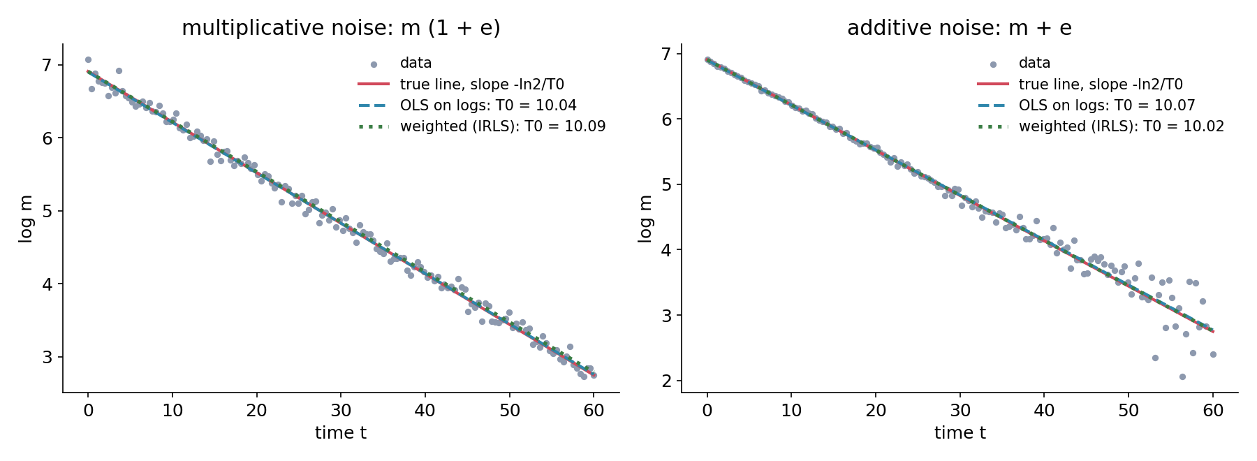
Same decay, two noise models, plotted in log scale. With multiplicative noise the scatter is uniform; with additive noise it fans out at late times, where the mass is small.

The cure is weighted least squares: give each point a weight equal to the inverse of its error variance, $w_i \propto 1/\operatorname{Var}(\text{error}_i) \propto m(t_i)^2$ . Since the true $m(t_i)$ is unknown, use the current fit and iterate (iteratively reweighted least squares, IRLS):

fit the line with all weights equal to 1;
set $w_i = \hat{m}(t_i)^2 = e^{2(a t_i + b)}$ ;
refit with these weights, repeat until stable.

At convergence this is (to first order) the same as fitting the original curve $m_0 2^{-t/T_0}$ directly to the masses by least squares, which is the right estimator for additive noise.

Which model is the right one? The data can tell you. After a first fit, look at the absolute residuals $\lvert m_i - \hat{m}_i\rvert$ . Under multiplicative noise they shrink with the mass; under additive noise they do not depend on it. A rank correlation (Spearman) between $\lvert m_i - \hat{m}_i\rvert$ and $\hat{m}_i$ above about 0.25 means multiplicative noise, so we keep plain least squares; otherwise we switch to IRLS. This is a tiny example of residual diagnostics, the habit of checking the assumptions of a model on its own errors.

The full solution

The submission uses only math, because a contest judge may not have NumPy. The core is one weighted line fit:

def weighted_line(t, y, w):
    sw = sum(w)
    mt = sum(wi * ti for wi, ti in zip(w, t)) / sw
    my = sum(wi * yi for wi, yi in zip(w, y)) / sw
    stt = sum(wi * (ti - mt) ** 2 for wi, ti in zip(w, t))
    sty = sum(wi * (ti - mt) * (yi - my) for wi, ti, yi in zip(w, t, y))
    a = sty / stt
    return a, my - a * mt

On top of it: half_life_ols (all weights 1), half_life_irls (30 reweighting rounds with $w_i = \hat m_i^2$ , normalised to avoid overflow), and half_life, which runs the Spearman test and picks one. With fewer than 8 points the test is meaningless and we keep the plain fit. Pay attention to the input order: each line is "mass time", not "time mass".

The --bench mode of solution.py simulates tests in the statement's ranges: $5 \le n < 1000$ , $T_0$ between 5 and 2000, $m_0$ up to 10 000, observation window of 1 to 4 half-lives (capped at $t \le 5000$ ), points with $m \le 1$ removed as the constraints require.

Results

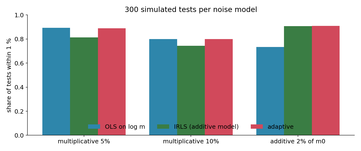
Share of 300 simulated tests per noise model that land within 1 % (same tests for every method):

Bar chart: plain least squares on the logs wins under multiplicative noise, IRLS wins under additive noise, and the adaptive rule matches the best of the two in every column.

approach	mult. 5 %	mult. 10 % (uniform)	additive, 2 % of $m_0$
least squares on $\log m$	0.893	0.800	0.733
IRLS, weights $\hat m^2$ (additive model)	0.813	0.743	0.907
weights $m_i$ from the raw data (tried, dropped)	0.80	0.75	0.70
adaptive (Spearman test picks the model)	0.890	0.800	0.910

Two lessons hide in this table. First, a weighting that is right for one noise model is wrong for the other: there is no universally best fit, only an estimator matched to the noise. Second, the remaining 10 to 20 % failures are not bugs: with a handful of points or a short observation window, the statistical uncertainty on the slope is itself larger than 1 %, and no method can beat it. (The standard error of the slope is about $\sigma / (\sqrt{n}\,\operatorname{sd}(t))$ : few points or a narrow time range make it large.)

The real tests are unknown to us; on the official sample, whose data are exact, every method returns $10.000$ (the sample output $10.01$ is within the 1 % tolerance too).

What to remember

Linearise with the right transform: exponential decay becomes a line in $\log m$ , and the half-life is $-\ln 2/\text{slope}$ .
A transform changes the noise as well as the curve. After $\log$ , an absolute error becomes $\varepsilon/m$ : small values become unreliable.
Weight each point by the inverse of its error variance; when that variance depends on the unknown fit, iterate (IRLS).
Diagnose the noise from the residuals instead of guessing: their behaviour against the fitted value tells you which model holds.
Benchmark on simulated data when the tests are hidden: generating your own tests with known answers is the only way to compare methods honestly.

Code complet (solution.py)

"""FAIO 2024 (Kazakhstan), day 1, problem C "Radioactive Decay".

Estimate the half-life T0 of m(t) = m0 * (1/2)^(t/T0) from n noisy pairs
"m t". Accepted if within 1 % of the truth.

    python solution.py < input.txt     -> prints T0 (the contest submission)
    python solution.py --bench         -> benchmark on simulated tests + figures

The submission uses only the standard library (math), as a contest judge may
not have numpy. Idea: log m is linear in t, slope = -ln2 / T0. Plain least
squares on the logs is optimal when the noise is multiplicative; when the
noise is additive, small masses get huge log errors, so we re-weight by the
fitted mass (iteratively reweighted least squares). A rank-correlation test
on the residuals decides which noise model the data show.
"""
import sys
from math import log, exp, isfinite

LN2 = log(2)


def weighted_line(t, y, w):
    """Weighted least squares fit y ~ a t + b (closed form of dL/da = dL/db = 0)."""
    sw = sum(w)
    mt = sum(wi * ti for wi, ti in zip(w, t)) / sw
    my = sum(wi * yi for wi, yi in zip(w, y)) / sw
    stt = sum(wi * (ti - mt) ** 2 for wi, ti in zip(w, t))
    sty = sum(wi * (ti - mt) * (yi - my) for wi, ti, yi in zip(w, t, y))
    a = sty / stt
    return a, my - a * mt


def half_life_ols(t, m):
    a, _ = weighted_line(t, [log(v) for v in m], [1.0] * len(t))
    return -LN2 / a


def half_life_irls(t, m, iters=30):
    """Minimises (approximately) sum (m_i - m0 2^(-t_i/T0))^2 : additive noise.
    The error on log m is about noise / m, so each point gets weight m_fit^2."""
    y = [log(v) for v in m]
    a, b = weighted_line(t, y, [1.0] * len(t))
    for _ in range(iters):
        w = [exp(2 * (a * ti + b)) for ti in t]
        s = max(w)
        a, b = weighted_line(t, y, [wi / s for wi in w])
    return -LN2 / a


def ranks(v):
    order = sorted(range(len(v)), key=v.__getitem__)
    r = [0.0] * len(v)
    for k, i in enumerate(order):
        r[i] = float(k)
    return r


def spearman(x, y):
    rx, ry = ranks(x), ranks(y)
    n = len(x); mx = my = (n - 1) / 2
    num = sum((a - mx) * (b - my) for a, b in zip(rx, ry))
    den = sum((a - mx) ** 2 for a in rx)
    return num / den


def half_life(t, m):
    """Adaptive: multiplicative noise -> plain log fit, additive -> IRLS."""
    if len(t) < 8:
        return half_life_ols(t, m)
    a, b = weighted_line(t, [log(v) for v in m], [1.0] * len(t))
    fit = [exp(a * ti + b) for ti in t]
    # multiplicative noise: |residual| grows with the mass; additive: it does not
    rho = spearman([abs(mi - fi) for mi, fi in zip(m, fit)], fit)
    T = half_life_ols(t, m) if rho > 0.25 else half_life_irls(t, m)
    return T if isfinite(T) and T > 0 else half_life_ols(t, m)


def main_stdin():
    data = sys.stdin.read().split()
    n = int(data[0])
    m = [float(data[1 + 2 * i]) for i in range(n)]
    t = [float(data[2 + 2 * i]) for i in range(n)]
    print(f"{half_life(t, m):.6f}")


# ------------------------------------------------------------------ benchmark
def bench():
    import numpy as np
    import matplotlib
    matplotlib.use("Agg")
    import matplotlib.pyplot as plt

    # sample test of the statement: exact data, T0 = 10
    t0, m0 = [0, 10, 20, 30, 40], [1000, 500, 250, 125, 62.5]
    print("sample:", round(half_life(t0, m0), 6))

    rng = np.random.default_rng(0)

    def gen(kind):
        n = int(rng.integers(5, 1000)); T0 = rng.uniform(5, 2000)
        M0 = rng.uniform(100, 10000)
        t = np.sort(rng.uniform(0, min(rng.uniform(1, 4) * T0, 5000), n))
        m = M0 * 0.5 ** (t / T0)
        if kind == "multiplicative 5%":
            m = m * np.exp(rng.normal(0, 0.05, n))
        elif kind == "multiplicative 10%":
            m = m * (1 + rng.uniform(-0.1, 0.1, n))
        else:
            m = m + rng.normal(0, 0.02 * M0, n)
        keep = m > 1                       # the statement guarantees m > 1
        return t[keep].tolist(), m[keep].tolist(), T0

    methods = {"OLS on log m": half_life_ols, "IRLS (additive model)": half_life_irls,
               "adaptive": half_life}
    kinds = ["multiplicative 5%", "multiplicative 10%", "additive 2% of m0"]
    table = {}
    for kind in kinds:
        tests = [gen(kind) for _ in range(300)]
        for name, f in methods.items():
            ok = [abs(f(t, m) - T0) / T0 < 0.01 for t, m, T0 in tests]
            table[(kind, name)] = np.mean(ok)
            print(f"{kind:20s} {name:22s} {np.mean(ok):.3f}")

    # figure 1: same decay, two noise models, in log scale
    plt.rcParams.update({"font.size": 12, "axes.spines.top": False, "axes.spines.right": False})
    t = np.linspace(0, 60, 150); T0, M0 = 10, 1000
    clean = M0 * 0.5 ** (t / T0)
    r = np.random.default_rng(3)
    mult = clean * np.exp(r.normal(0, 0.08, t.size))
    add = clean + r.normal(0, 8, t.size)
    fig, axs = plt.subplots(1, 2, figsize=(12, 4.4), dpi=150)
    for ax, m, title in [(axs[0], mult, "multiplicative noise: m (1 + e)"),
                         (axs[1], add, "additive noise: m + e")]:
        k = m > 1
        ax.scatter(t[k], np.log(m[k]), s=12, color="#8d99ae", label="data")
        ax.plot(t, np.log(clean), color="#d1495b", lw=2, label="true line, slope -ln2/T0")
        a, b = np.polyfit(t[k], np.log(m[k]), 1)
        ax.plot(t, a * t + b, "--", color="#2e86ab", lw=2,
                label=f"OLS on logs: T0 = {-np.log(2)/a:.2f}")
        Ti = half_life_irls(t[k].tolist(), m[k].tolist())
        ax.plot(t, np.log(M0) - np.log(2) * t / Ti, ":", color="#3a7d44", lw=2.5,
                label=f"weighted (IRLS): T0 = {Ti:.2f}")
        ax.set_title(title); ax.set_xlabel("time t"); ax.set_ylabel("log m")
        ax.legend(frameon=False, fontsize=10)
    fig.tight_layout(); fig.savefig("figures/log_scale.png", facecolor="white")

    # figure 2: success rate per method and noise model
    fig, ax = plt.subplots(figsize=(10, 4.2), dpi=150)
    wdt = 0.26; cols = ["#2e86ab", "#3a7d44", "#d1495b"]
    for j, name in enumerate(methods):
        ax.bar(np.arange(3) + (j - 1) * wdt, [table[(k, name)] for k in kinds], wdt,
               label=name, color=cols[j])
    ax.set_xticks(range(3)); ax.set_xticklabels(kinds)
    ax.set_ylim(0, 1); ax.set_ylabel("share of tests within 1 %")
    ax.set_title("300 simulated tests per noise model")
    ax.legend(frameon=False, ncol=3, loc="lower center")
    fig.tight_layout(); fig.savefig("figures/benchmark.png", facecolor="white")
    print("figures written")


if __name__ == "__main__":
    bench() if "--bench" in sys.argv else main_stdin()