IOAI Training: Learn AI by solving problems

The problem in brief

You are shown the first two sentences of the abstracts of two arXiv papers and must say which of the two was submitted later. For training you get 37 177 papers, each with its two opening sentences, its exact submission date (2000 to April 2025) and its arXiv categories, sampled so that each of the 140 categories has at least 10 papers per year. You also get, as a bonus, the daily number of papers per category (the data of the home assignment). The test has 24 050 pairs built from other papers, drawn evenly over 2000 to 2025, and in every pair the two papers are at least two years apart. You answer 1 if the second paper is newer, 0 if the first one is.

The data comes from the Kaggle competition archive. The test labels are private and we never submitted anything, so all scores below come from our own validation on held-out training papers.

How you are scored

Plain accuracy over the pairs:

\text{accuracy} = \frac{1}{N}\sum_{k=1}^{N} \mathbf 1\big[\hat\ell_k = \ell_k\big].

Guessing gives 0.50. The organisers turned the public-leaderboard accuracy into points with four benchmarks: 55 % = 30 points, 60 % = 60, 65 % = 90, 70 % = 120 (the maximum), plus points for the final rank. On the public leaderboard of the archive, the best entry is 0.718 and the next one 0.705.

First look at the data

The training papers are spread evenly over time (from about 1 100 per year in 2000 to 1 550 per year after 2017), and every paper is a short text of about 320 characters. Nothing like a date or an arXiv identifier is in the text, so the date has to be guessed from how and about what people wrote.

Two simple style signals are almost useless: the text length gives 0.54 pair accuracy and the number of $ signs (LaTeX formulas) gives 0.51. The signal is in the vocabulary, as the next figure shows.

To validate we keep 20 % of the training papers aside (7 436 papers) and build 20 000 random pairs from them with the same rule as the test: the two dates must be at least two years apart. With 20 000 pairs the standard error of an accuracy near 0.7 is about 0.3 points, so differences of 1 point are real.

A first baseline

Turn the pairwise question into a regression. Instead of learning on pairs, learn one function $f(\text{text}) \approx$ date, in years, on the 37 000 dated papers, and answer

\hat\ell = \mathbf 1\big[f(\text{second}) > f(\text{first})\big].

The simplest $f$ is a ridge regression on TF-IDF features, which gives 0.69 with word 1-2 grams and 0.70 with word and character n-grams together, already at the top benchmark.

Words that date a paper

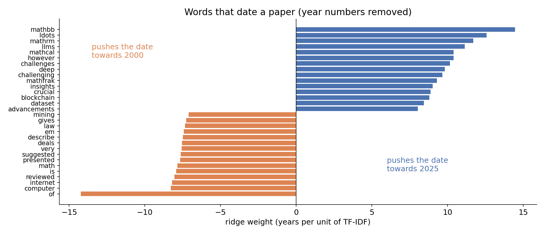
The weights read like a history of science writing. Old papers talk about the internet, the web, computer and mining, and use plain verbs like we describe, is discussed, deals with. New papers say deep, dataset, blockchain, LLMs, and have the inflated vocabulary of the last few years: crucial, insights, advancements, challenges. Many of the strongest "new" features are LaTeX commands (\mathbb, \mathcal, \mathrm): arXiv abstracts started to carry inline LaTeX much more often in recent years. Each of these words is a small clue; together they place a paper in time to within about five years.

The key idea

A pair is decided by the difference of two noisy date estimates, so what matters is ranking, not calibration. Look at the left panel below. The predicted dates are strongly pulled towards the middle (a 2001 paper is predicted around 2010, a 2024 paper around 2018). Ridge regression shrinks uncertain predictions towards the mean, so the mean absolute error is a poor 5 years. But this bias is almost monotonic: older papers still get lower predictions on average, and a monotonic distortion does not change which of two papers gets the larger value. That is why a model with a 5-year error can still answer most pairs correctly.

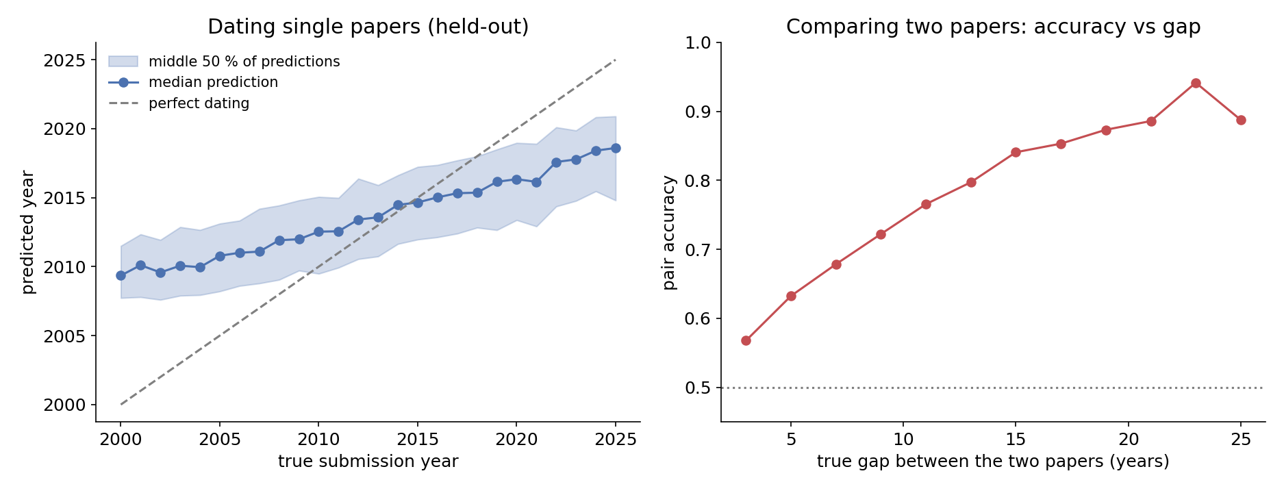
Dating single papers and accuracy by gap

The right panel shows the other side of the same coin. If the prediction error of each paper is roughly Gaussian with spread $\sigma$ , then for two papers $\Delta$ years apart

P(\text{correct}) \approx \Phi\!\left(\frac{\Delta}{\sqrt 2\,\sigma}\right),

which grows with the gap. Pairs 2 to 4 years apart are barely better than a coin (0.57), pairs more than 14 years apart are 0.87 right. Since the test pairs have random gaps of at least 2 years, the only way to gain is to shrink $\sigma$ , that is to date each paper better, and to combine models whose errors are different, because averaging two independent errors divides the variance.

So we add a second dater of a different nature: a small pretrained sentence encoder, all-MiniLM-L6-v2 (22 M parameters), fine-tuned to output the date. TF-IDF sees exact words; the encoder sees meaning ("transformer-based language model" and "LLM" are close for it) and generalises to phrasings the ridge never saw. Used frozen (embeddings + ridge or MLP), MiniLM is worse than TF-IDF (0.65 to 0.67), because generic sentence embeddings are trained to ignore style and keep topic. Fine-tuned end to end, it learns what matters for dating and beats TF-IDF.

We also tried to use the shape of the problem more cleverly: a 26-class logistic regression gives a full distribution $p(\text{year}\mid\text{text})$ for each paper, and the probability that B is newer given that the gap is at least 2 years can be computed exactly,

P(B \succ A) \propto \sum_{y_B - y_A \ge 2} p_A(y_A)\, p_B(y_B).

It gave 0.702, the same as comparing expected years (0.703). The constraint carries little information once the predictions are this noisy.

The full solution

Target: the fractional submission year, e.g. 2013.42.
Dater 1: TF-IDF of words (1-2 grams, 200 000 features) and of characters (2-5 grams inside words, 200 000 features), sublinear term frequency, ridge regression with $\alpha = 3$ .
Dater 2: all-MiniLM-L6-v2 with a mean-pooling layer and a linear head, trained 3 epochs with AdamW (learning rate $5\times10^{-5}$ , one-cycle schedule), smooth L1 loss on the standardised year, batches of 16 texts padded to 112 tokens:

h = self.enc(**e).last_hidden_state                 # (batch, tokens, 384)
k = e['attention_mask'].unsqueeze(-1).float()
date = self.head((h * k).sum(1) / k.sum(1))         # mean over real tokens, then linear

Blend: average the two predicted years (weights 0.4 to 0.6 all give the same accuracy within 0.1 point).
Answer: 1 if the blended date of the second paper is larger. For the test, both daters are retrained on all 37 177 papers.

What we did not use: the categories and the time series. The categories are not given for test papers, so they could only enter through a model that predicts the category from the text, and the date regressors already learn the topic implicitly (a paper about LLMs is new whatever its category). The time series tells when each category was busy, but the test papers were drawn evenly over time within each category, so it adds little.

Results

Accuracy on 20 000 held-out pairs (gap of at least 2 years) built from 20 % of the training papers; the official test labels are private.

approach	pair accuracy
text length	0.538
number of `$` signs	0.514
frozen MiniLM embeddings + ridge	0.652
frozen MiniLM embeddings + MLP	0.665
TF-IDF words + ridge	0.693
TF-IDF characters + ridge	0.698
TF-IDF words + characters + ridge	0.704
26-class logistic regression, expected year	0.703
same, exact "gap at least 2 years" probability	0.702
fine-tuned MiniLM regressor	0.713
average of TF-IDF ridge and fine-tuned MiniLM (final)	0.724

The final blend reaches 0.724 on our held-out pairs, above the top benchmark (70 %, maximum points) and level with the best public-leaderboard entry (0.718). A held-out split from the training papers is a fair but not perfect stand-in for the test: the test papers were sampled differently (400 per category spread over time), and our ridge model dates test papers about 0.8 years later on average than validation papers, so the test mix leans a little more towards recent years.

What to remember

Pairwise questions can be answered with a pointwise model. Learn a score per item (here a date) and compare scores. You use every labelled item once instead of building pairs, and the comparison is automatically consistent.
For ranking, bias does not matter, noise does. A regressor that shrinks everything towards 2012 still ranks papers well. Measure what the task measures (pair accuracy), not the regression error.
Look at the weights of a linear model. They show you what the data is really about: here, the drift of scientific vocabulary and of LaTeX habits.
Frozen embeddings are not always better than TF-IDF. Generic sentence encoders are trained to ignore the style cues that date a text; fine-tuning on the real target fixes that.
Blend models that make different mistakes. A bag of n-grams and a fine-tuned encoder err differently, and their plain average beats both by about 1 to 2 points.

"""Which Paper Is Newer? (Kazakhstan AI Olymp 2025, final, day 2).

Idea: turn the pairwise question into a regression. Learn a "dating" function
f(text) ~ submission date (in years) on the 37k dated training papers, then answer
"is B newer than A?" by comparing f(B) with f(A).
  * f1: ridge regression on TF-IDF of words (1-2 grams) + characters (2-5 grams)
  * f2: all-MiniLM-L6-v2 fine-tuned as a regressor (mean pooling + linear head)
  * final score = average of the two predictions (both are in years)

Data: kaggle competition "kazakhstan-respa-final-day-2-late-competition"
      (train_sentences.csv, test_sentences.csv). Encoder: sentence-transformers/all-MiniLM-L6-v2.
Usage: python solution.py val    -> 80/20 split, accuracy on 20k held-out pairs (gap >= 2 years)
       python solution.py test   -> train on everything, write submission.csv (not submitted)
Runtime: ~3 min (TF-IDF) + ~12 min (fine-tuning on Apple MPS); peak memory ~2 GB.
"""
import sys, numpy as np, pandas as pd, scipy.sparse as sp, torch
from sklearn.feature_extraction.text import TfidfVectorizer
from sklearn.linear_model import Ridge
from sklearn.model_selection import train_test_split
from transformers import AutoTokenizer, AutoModel

torch.set_num_threads(2)
DEV = 'mps' if torch.backends.mps.is_available() else 'cpu'
if DEV == 'mps':
    torch.mps.set_per_process_memory_fraction(0.1)      # hard cap on GPU memory
ENCODER = 'sentence-transformers/all-MiniLM-L6-v2'
MAXLEN, BS, EPOCHS, LR = 112, 16, 3, 5e-5


def load():
    t = pd.read_csv('train_sentences.csv')
    d = pd.to_datetime(t.submitted_date)
    t['y'] = d.dt.year + (d.dt.dayofyear - 1) / 366     # fractional year
    return t


# ------------------------------------------------------------------ model 1: TF-IDF + ridge
def tfidf_ridge(train_txt, y, *predict_txt):
    w = TfidfVectorizer(ngram_range=(1, 2), min_df=2, sublinear_tf=True, max_features=200000)
    c = TfidfVectorizer(analyzer='char_wb', ngram_range=(2, 5), min_df=3, sublinear_tf=True, max_features=200000)
    X = sp.hstack([w.fit_transform(train_txt), c.fit_transform(train_txt)]).tocsr()
    m = Ridge(alpha=3).fit(X, y)
    return [m.predict(sp.hstack([w.transform(p), c.transform(p)]).tocsr()) for p in predict_txt]


# ------------------------------------------------------------------ model 2: fine-tuned encoder
class Regressor(torch.nn.Module):
    def __init__(self, enc):
        super().__init__(); self.enc = enc
        self.head = torch.nn.Linear(enc.config.hidden_size, 1)

    def forward(self, **e):
        h = self.enc(**e).last_hidden_state
        k = e['attention_mask'].unsqueeze(-1).float()
        return self.head((h * k).sum(1) / k.sum(1)).squeeze(-1)   # mean pooling -> date


def encoder_regression(train_txt, y, *predict_txt):
    torch.manual_seed(0)
    tok = AutoTokenizer.from_pretrained(ENCODER)
    model = Regressor(AutoModel.from_pretrained(ENCODER)).to(DEV)
    # fixed-length padding: constant tensor shapes keep the MPS memory cache flat
    batch = lambda txt: tok(list(txt), padding='max_length', max_length=MAXLEN,
                            truncation=True, return_tensors='pt').to(DEV)
    X, Y = np.asarray(train_txt), ((np.asarray(y) - 2012.5) / 7.5).astype(np.float32)
    steps = EPOCHS * (len(X) // BS)
    opt = torch.optim.AdamW(model.parameters(), lr=LR, weight_decay=0.01)
    sch = torch.optim.lr_scheduler.OneCycleLR(opt, max_lr=LR, total_steps=steps,
                                              pct_start=0.06, anneal_strategy='linear')
    for ep in range(EPOCHS):
        model.train(); perm = np.random.RandomState(ep).permutation(len(X))
        for b in range(len(X) // BS):
            idx = perm[b * BS:(b + 1) * BS]
            out = model(**batch(X[idx]))
            loss = torch.nn.functional.smooth_l1_loss(out, torch.tensor(Y[idx], device=DEV))
            loss.backward(); opt.step(); sch.step(); opt.zero_grad()
        print(f'  epoch {ep} done, last loss {loss.item():.3f}', flush=True)
    del opt
    model.eval(); res = []
    with torch.no_grad():
        for txt in predict_txt:
            txt = np.asarray(txt)
            p = np.concatenate([model(**batch(txt[i:i + 32])).cpu().numpy() for i in range(0, len(txt), 32)])
            res.append(p * 7.5 + 2012.5)
    return res


def pair_accuracy(p, y, pairs):
    a, b = pairs
    return np.mean((p[b] > p[a]) == (y[b] > y[a]))


if __name__ == '__main__':
    t = load()
    if sys.argv[1:] == ['val']:
        tr, va = train_test_split(t, test_size=0.2, random_state=0)
        yv = va.y.values
        rng = np.random.RandomState(0)                 # random pairs with a >= 2 year gap, like the test
        i, j = rng.randint(0, len(va), 60000), rng.randint(0, len(va), 60000)
        keep = np.abs(yv[i] - yv[j]) >= 2
        pairs = (i[keep][:20000], j[keep][:20000])
        p1, = tfidf_ridge(tr.sentences, tr.y, va.sentences)
        p2, = encoder_regression(tr.sentences, tr.y, va.sentences)
        for name, p in [('tfidf ridge', p1), ('fine-tuned MiniLM', p2), ('average', (p1 + p2) / 2)]:
            print(f'{name:18s} pair accuracy {pair_accuracy(p, yv, pairs):.4f}  MAE {np.abs(p - yv).mean():.2f} y')
    else:
        s = pd.read_csv('test_sentences.csv')
        a1, b1 = tfidf_ridge(t.sentences, t.y, s.first_sentence, s.second_sentence)
        a2, b2 = encoder_regression(t.sentences, t.y, s.first_sentence, s.second_sentence)
        label = ((b1 + b2) > (a1 + a2)).astype(int)    # 1 = the second paper is newer
        pd.DataFrame({'ID': s.ID, 'label': label}).to_csv('submission.csv', index=False)
        print('wrote submission.csv (not submitted); share of 1:', label.mean())