IOAI Training: Learn AI by solving problems

The problem in brief

Six robots live in small rooms: a 6 x 6 floor surrounded by walls, scattered with keys, balls and boxes of six colours, plus some coloured "tokens". Each robot is given an English mission of one of three kinds (go to an object, pick up an object, put one object next to another), phrased in many ways ("grab the blue key", "collect the blue key"...). You see one snapshot at a random moment of the robot's work: the room, the robot's position and facing direction, the mission and what it carries. You must predict its next action among six (up, down, left, right, pick up, drop). The robots do not always take shortest paths, and each robot has its own habits. You get 60 000 labelled snapshots (10 000 per robot); the notebook must run in 5 minutes on the hidden test set.

The organisers published the graded splits after the contest, so we report our final score on leaderboard B (3 600 snapshots, the split that decided the ranking). All choices were made on a 10 % holdout of the training set.

How you are scored

Accuracy is computed separately for each robot, then averaged, on a 0 to 100 scale:

\text{score} = \frac{100}{6}\sum_{r=0}^{5} \frac{\#\{\text{correct predictions for robot } r\}}{\#\{\text{snapshots of robot } r\}} .

Reference points, from the official grader's runbook (code/grading-original/RUNBOOK.md in the IOAI-2026 repository): the baseline that always answers "up" scores 20.58 on leaderboard B, and the authors' own solution, per-robot neural networks, scores 71.14. The official ranking then normalises each task (IOAI 2026 rules, technical appendix): $100\,(\text{raw} - \text{Min})/(\text{Max} - \text{Min})$ , where Min is the baseline and Max the larger of 0.9 times the committee's solution and the best contestant's raw score. In the published results the best normalised score on this task was 86.2.

First look at the data

The first thing to understand is what the robot is trying to reach, because the mission alone does not explain the actions. Counting tokens gives the key: every room has either 6 tokens, exactly one of which has the robot's own colour (colour id = robot id), or 5 tokens with none of the robot's colour, and the robot is never seen carrying a token. So each robot first collects its own token, which disappears, and only then does its mission. In about half of the snapshots (48 %), the robot is still heading for its token.

This gives a sequence of sub-goals that you can compute from the snapshot alone:

own token still on the floor: walk next to it, face it, pick it up;
"go to X": walk next to X;
"pick up X": walk next to X, face it, pick it up;
"put X next to Y": pick up X, then walk until X can be dropped on a free cell next to Y, and drop it.

Then look at what the robots actually do in a clean situation. In the right panel below, the robot's own token is straight above, two or more cells away, with a free path. If the robot already faces up, it goes up 70 % of the time. If it faces down, it goes up 70 % of the time too, but otherwise mostly answers "left" or "right": exactly what a robot that can only turn by 90 degrees would do to turn around, once the turns are written as absolute directions. And there is real noise: "pick up" in front of an empty cell, or "left" when facing the token (the left panel's robot is next to its token, facing it, and moves "left" into it instead of picking it up). About 18 % of all "pick up" actions are performed in front of nothing that can be picked up.

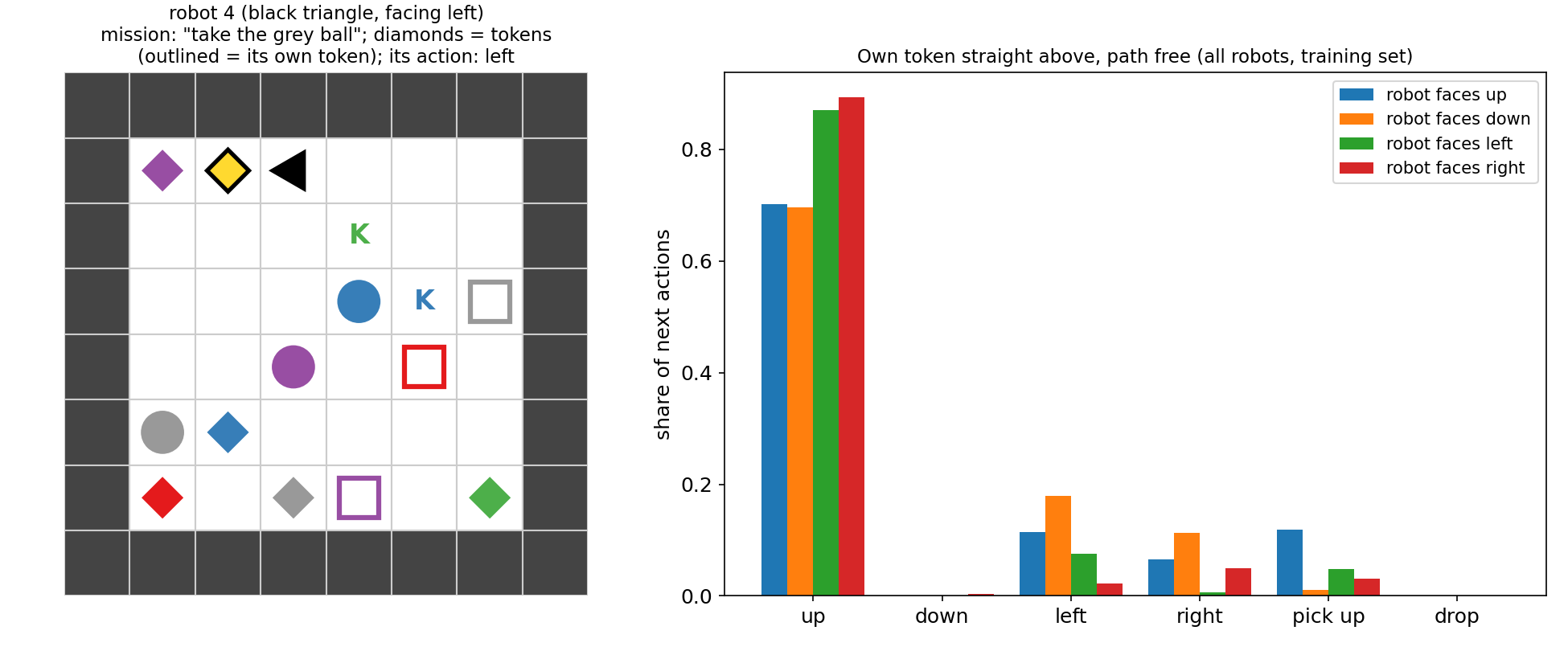
A training snapshot, and the next-action distribution in one clean situation

So the best possible score is far from 100: the behaviour is partly random, and the job is to predict the most likely action in each situation.

A first baseline

Always answering "up" gives 20.6 (the official baseline). Answering with the shortest-path move towards the current sub-goal is much better, but the hand-written rules quickly become a maze of exceptions (turns, blocked cells, ties between two equally short moves). It is more effective to compute features that describe the situation and let a model learn each robot's habits:

the sub-goal type (token, reach, pick, pick-for-put, drop) and the mission type;
the BFS distance (moves through empty cells) from the robot to a cell next to the sub-goal, and the change of that distance for each of the four moves (a move into an obstacle only turns the robot, so its distance does not change);
what is in front of the robot and on each of its four sides; whether it faces its target; whether the cell in front is a valid place to drop;
the offset $(\Delta r, \Delta c)$ to the target, its Manhattan distance, the direction the robot faces, what it carries.

A gradient-boosted tree model (HistGradientBoostingClassifier, 500 trees, robot id as a categorical feature) on these 37 features reaches 63.8 on the holdout and 61.9 on leaderboard B. Training one model per robot is worse (61.1 on the holdout): the robots share most of their behaviour, so splitting the data divides it by six for little gain.

The key idea

Turn a perception problem into a planning one. A raw 8 x 8 x 2 grid plus a sentence is hard to learn from: the model would have to discover on its own that a token of the robot's colour matters, that a "put" mission has two phases, and what a shortest path is. Computing the current sub-goal and the BFS distances by hand injects exactly the structure of the task. After that, what remains to learn is small: each robot's habits (how often it turns, which of two equally good moves it prefers, how noisy it is), which a model can estimate from 10 000 examples per robot.

The second ingredient is to keep the spatial picture as well, because features cannot list every relevant configuration (a box next to the target, a wall around the corner). The final model therefore combines both:

a small CNN reads the grid as 26 one-hot channels: object type per cell, "is my own token", "is mission object 1 or 2", plus the direction, carrying state, mission type and robot id broadcast to every cell;
its output is concatenated with the standardised hand-made features;
a dense layer produces six separate 6-way outputs, one per robot, and we read the one of the robot in the snapshot. The robots share the whole network except the last layer, which is a cheap way to get "per-robot models" without dividing the data.

The full solution

Parse the mission with a regular expression (colour + object, one or two of them) and its first word (go / pick / put family).
Compute the sub-goal and the 37 features (BFS on the 6 x 6 floor, at most 36 cells, so this is instant).
Build the 26-channel grid encoding.
Train the CNN + features network for 18 epochs with AdamW and a one-cycle learning rate up to $2 \times 10^{-3}$ , batches of 256, on all 60 000 snapshots (about 6 minutes on 2 CPU threads, much less on the contest GPU).
Predict the argmax of the robot's own output head.

z = self.f(torch.cat([self.c(grid).flatten(1), feats], 1)).view(-1, 6, 6)
logits = z[torch.arange(len(robot)), robot]      # the head of this snapshot's robot

We also tried an egocentric grid (re-centred on the robot, 15 x 15), a common trick in gridworlds. It overfitted (holdout 65.9 at best, then falling to 64.8), probably because the walls' absolute position matters in such a small room.

Results

Mean per-robot accuracy x 100. Holdout = 10 % of the training set; leaderboard A and B are the official hidden test splits, scored with the official metric.

approach	holdout	leaderboard A	leaderboard B
always "up" (official baseline)		20.81	20.58
boosted trees on 37 sub-goal features	63.8	61.7	61.9
same, one model per robot	61.1
egocentric CNN + features (12 epochs)	64.8
CNN on the grid + features, one head per robot (final)	66.5	63.2	62.2
authors' solution (per-robot MLPs, from the runbook)		72.03	71.14

Our final model scores 62.2 on leaderboard B, three times the baseline but 9 points below the authors' 71.1. With the official normalisation, if the committee's reference is the authors' 71.14 (so Max = 0.9 x 71.14 = 64.0), 62.2 would be worth about 96 normalised points, above the best contestant's 86.2; but the exact committee reference is not published, so treat that conversion as indicative.

Two honest observations. First, the official test splits are about 3 to 4 points harder than our random holdout (also true for the public test file), so the training rows are not a perfect preview of the test rows; we did not find out why (layouts never repeat between train and test, and the mix of sub-goals is the same). Second, the drop phase of "put" missions is our weakest part (about 50 % accuracy on leaderboard B against 67 % in the token phase): deciding where a robot will choose to drop its object is the hardest pattern to read from a single snapshot.

What to remember

Find the hidden sub-goal first. Counting tokens revealed that every robot collects its own-coloured token before its mission; without that, half the snapshots look random.
Inject the planning you know. BFS distances and "what each move would change" turn a hard perception problem into an easy tabular one; the model then only has to learn habits and noise.
Know the ceiling. When behaviour is stochastic, 100 % is impossible: estimate how noisy the labels are (here, pick-ups in front of empty cells) before chasing the last points.
Share, then specialise. One network with a separate output head per robot uses all the data for the common behaviour and still lets each robot differ, which beat one model per robot.
Validate like the test. A random holdout overestimated the test score by 3 to 4 points; when the organisers warn about "new combinations", expect a gap and keep a margin.

"""Robot Chasing (IOAI 2026, day 1): predict the next action of six gridworld robots.

1. Parse the mission (go to / pick up / put next to, object + colour).
2. Work out the robot's current sub-goal: its own token first (the token whose colour is the
   robot id; it disappears once picked), then the mission object, then the drop target.
3. Hand-made features: BFS distance to the sub-goal from the robot and from each neighbour,
   what is in front, what is on each side, whether the robot faces its target...
4. A small CNN over the one-hot 8x8 grid (+ mission/target channels) concatenated with those
   features, with one 6-way output per robot.  Trained on all 60,000 training rows.
Usage: python solution.py val 12   (90/10 holdout)   |   python solution.py full 18  (predict LB A/B)
Data layout: data/public/train/observations.json + data/public/train_answers.json, data/private/...
"""
import json, sys, time, re
from collections import deque
import numpy as np, pandas as pd, torch, torch.nn as nn, torch.nn.functional as F

# ---------------- parsing ----------------
COL = {"red": 0, "green": 1, "blue": 2, "purple": 3, "yellow": 4, "grey": 5}
OBJ = {"key": 5, "ball": 6, "box": 7}
def task(m):
    w = m.split()[0]
    if w in ("put", "place") or m.startswith("move the"): return "put"
    if w in ("pick", "take", "grab", "collect"): return "pick"
    return "go"
def pairs(m):
    return [(OBJ[o], COL[c]) for c, o in re.findall(r"\b(red|green|blue|purple|yellow|grey) (key|ball|box)\b", m)]
def load(split, root="data"):
    pub = split in ("train", "pretest", "pretrain")
    base = f"{root}/{'public' if pub else 'private'}"
    O = json.load(open(f"{base}/{split}/observations.json")); Y = json.load(open(f"{base}/{split}_answers.json"))
    return O, Y
def find(img, oc):
    return [(r, c) for r in range(8) for c in range(8) if tuple(img[r][c]) == oc]
def robot(img):
    for r in range(8):
        for c in range(8):
            if img[r][c][0] == 10: return r, c

# ---------------- sub-goal + features ----------------

D = [(-1, 0), (1, 0), (0, -1), (0, 1)]
INF = 30

def bfs(img, starts):
    """Distance (moves through empty cells) from every cell to the nearest cell in `starts`."""
    dist = np.full((8, 8), INF)
    q = deque()
    for s in starts:
        dist[s] = 0; q.append(s)
    while q:
        r, c = q.popleft()
        for dr, dc in D:
            nr, nc = r + dr, c + dc
            if dist[nr, nc] == INF and img[nr][nc][0] == 1:
                dist[nr, nc] = dist[r, c] + 1; q.append((nr, nc))
    return dist

def goal(o):
    """Current sub-goal: (kind, object cell). kind in token / reach / pick / drop."""
    img, rid, m = o["image"], o["robot_id"], o["mission"]
    tok = find(img, (11, rid))
    if tok: return "token", tok[0]
    t, P = task(m), pairs(m)
    car = tuple(o["carrying"]) if o["carrying"] else None
    if t == "go": L = find(img, P[0]); return "reach", (L[0] if L else None)
    if t == "pick": L = find(img, P[0]); return "pick", (L[0] if L else None)
    if car == P[0]: L = find(img, P[1]); return "drop", (L[0] if L else None)
    L = find(img, P[0]); return "pickput", (L[0] if L else None)

KINDS = ["token", "reach", "pick", "pickput", "drop"]
CELL = {1: 0, 2: 1, 5: 2, 6: 2, 7: 2, 10: 3, 11: 4}

def featurize(o):
    img = o["image"]; rr, rc = robot(img); d = o["direction"]
    kind, g = goal(o)
    f = {"robot": o["robot_id"], "kind": KINDS.index(kind), "dir": d, "task": ["go", "pick", "put"].index(task(o["mission"])),
         "carry": 0 if not o["carrying"] else (2 if o["carrying"][0] == 11 else 1), "goal_found": int(g is not None)}
    fr, fc = rr + D[d][0], rc + D[d][1]
    f["front"] = CELL[img[fr][fc][0]]
    if g is None:
        f.update(dr=0, dc=0, man=-1, facing_goal=0, cur=INF)
        for a in range(4): f.update({f"cell{a}": CELL[img[rr + D[a][0]][rc + D[a][1]][0]], f"nd{a}": INF, f"delta{a}": 0, f"face{a}": 0})
        f["front_drop_ok"] = 0
        return f
    gr, gc = g
    f.update(dr=gr - rr, dc=gc - rc, man=abs(gr - rr) + abs(gc - rc), facing_goal=int((fr, fc) == g))
    if kind == "drop":
        # cells next to the target where the carried object may land; the robot must stand next to such a cell
        land = [(gr + a, gc + b) for a, b in D if img[gr + a][gc + b][0] == 1 or (gr + a, gc + b) == (rr, rc)]
        targets = [(x + a, y + b) for x, y in land for a, b in D if img[x + a][y + b][0] in (1, 10) and (x + a, y + b) != g]
        f["front_drop_ok"] = int((fr, fc) in land and img[fr][fc][0] == 1)
    else:
        targets = [(gr + a, gc + b) for a, b in D if img[gr + a][gc + b][0] in (1, 10)]
        f["front_drop_ok"] = 0
    tmp = [row[:] for row in img]; tmp[rr][rc] = [1, 0]
    dist = bfs(tmp, targets)
    f["cur"] = dist[rr, rc]
    for a in range(4):
        nr, nc = rr + D[a][0], rc + D[a][1]
        cell = img[nr][nc][0]
        f[f"cell{a}"] = CELL[cell]
        f[f"is_goal{a}"] = int((nr, nc) == g)
        nd = dist[nr, nc] if cell == 1 else dist[rr, rc]  # blocked moves only turn
        f[f"nd{a}"] = nd; f[f"delta{a}"] = nd - dist[rr, rc]
        f[f"face{a}"] = int((nr, nc) == g) if kind != "drop" else int(cell == 1 and (nr, nc) in land)
        f[f"toward{a}"] = int((D[a][0] and (gr - rr) * D[a][0] > 0) or (D[a][1] and (gc - rc) * D[a][1] > 0))
    return f

def table(O):
    import pandas as pd
    return pd.DataFrame([featurize(o) for o in O]).fillna(0)

# ---------------- model ----------------
torch.set_num_threads(2); torch.manual_seed(0)
OBJS=[1,2,5,6,7,10,11]
def encode(O):
    G=np.zeros((len(O),26,8,8),np.float32)
    for k,o in enumerate(O):
        im=np.asarray(o['image']); ob,co=im[:,:,0],im[:,:,1]
        for i,v in enumerate(OBJS): G[k,i]=ob==v
        G[k,7]=(ob==11)&(co==o['robot_id'])
        P=pairs(o['mission'])
        for j,(oo,cc) in enumerate(P[:2]): G[k,8+j]=(ob==oo)&(co==cc)
        G[k,10+o['direction']]=1
        car=o['carrying']; G[k,14+(0 if car is None else (1 if tuple(car)==tuple(P[0]) else 2))]=1
        G[k,17+['go','pick','put'].index(task(o['mission']))]=1
        G[k,20+o['robot_id']]=1
    return torch.tensor(G)
class Net(nn.Module):
    def __init__(s,nf):
        super().__init__()
        s.c=nn.Sequential(nn.Conv2d(26,64,3,padding=1),nn.ReLU(),nn.Conv2d(64,64,3,padding=1),nn.ReLU(),nn.Conv2d(64,64,3,padding=1),nn.ReLU())
        s.f=nn.Sequential(nn.Linear(64*64+nf,256),nn.ReLU(),nn.Dropout(0.2),nn.Linear(256,6*6))
    def forward(s,g,f,r):
        z=s.f(torch.cat([s.c(g).flatten(1),f],1)).view(-1,6,6)   # one 6-way output per robot
        return z[torch.arange(len(r)),r]
def feats(name):
    O,_=load(name); return table(O).astype(float)
if __name__=='__main__':
    O,Y=load('train'); G=encode(O); Xf=feats('train'); mu,sd=Xf.mean(),Xf.std()+1e-6
    Ft=torch.tensor(((Xf-mu)/sd).values,dtype=torch.float32); R=torch.tensor([o['robot_id'] for o in O]); Yt=torch.tensor(Y)
    rng=np.random.default_rng(0); m=torch.tensor(rng.random(len(Y))<0.9)
    full = len(sys.argv)>1 and sys.argv[1]=='full'
    if full: m[:]=True
    net=Net(Ft.shape[1]); EP=int(sys.argv[2]) if len(sys.argv)>2 else 12
    opt=torch.optim.AdamW(net.parameters(),1e-3,weight_decay=1e-4); idx=torch.where(m)[0]
    sched=torch.optim.lr_scheduler.OneCycleLR(opt,2e-3,total_steps=EP*(len(idx)//256+1))
    def mpra(p,y,r): return 100*np.mean([(p[r==k]==y[r==k]).float().mean().item() for k in range(6)])
    t=time.time()
    for ep in range(EP):
        net.train(); perm=idx[torch.randperm(len(idx))]
        for b in perm.split(256):
            loss=F.cross_entropy(net(G[b],Ft[b],R[b]),Yt[b]); opt.zero_grad(); loss.backward(); opt.step(); sched.step()
        if not full:
            net.eval(); h=torch.where(~m)[0]
            with torch.no_grad(): p=net(G[h],Ft[h],R[h]).argmax(1)
            print(ep+1,'holdout',round(mpra(p,Yt[h],R[h]),2),f'{time.time()-t:.0f}s',flush=True)
    if full:
        net.eval()
        for s in ['test_leaderboard_a','test_leaderboard_b']:
            O2,Y2=load(s); G2=encode(O2); F2=torch.tensor(((feats(s)-mu)/sd).values,dtype=torch.float32); R2=torch.tensor([o['robot_id'] for o in O2])
            with torch.no_grad(): p=net(G2,F2,R2).argmax(1)
            json.dump(p.tolist(),open(f'pred_{s}.json','w')); print(s,round(mpra(p,torch.tensor(Y2),R2),2))