Theory

The problem in brief

This is the written theory paper of INAIO 2026 Stage 2 (the PDF header says "Stage 3, Jan 18, 2026", but the file is the April Stage 2 theory test). It is worth 60 points and has three sections. Section A (Foundations, 20 points) asks for short NumPy code, a physics-based trajectory fit, reverse-engineering two well-known metrics from code, debugging a DNA motif scanner and designing two dashboards. Section B (ML theory, 20 points) is about choosing classifiers from a scatter plot, regularised regression, clustering sparse text, and practical evaluation traps. Section C (20 points) asks for four end-to-end system designs.

All computational answers were checked in Python: the matrix identities on random matrices, the trajectory against a numerical ODE solver, the fixed motif scanner against a brute-force reference on 20 000 random sequences, and the AUC/precision claim on a simulated classifier (see the solution code).

How you are scored

Points are printed next to every sub-question, from 1 to 2 points each. The graders read answers generously but expect the right mathematical object, the right function or the right justification. A4 gives 1 point per correctly identified bug, up to 4. No pass mark is published, so the target is a complete, justified answer to each sub-question.

Section A: Foundations

A1. Matrix expressions with a minimal toolbox

(a) Expand $\lVert A(u-v)\rVert^2 = (u-v)^\top A^\top A (u-v) = u^\top A^\top A u - 2u^\top A^\top A v + v^\top A^\top A v$, using that $u^\top A^\top A v$ is a scalar and so equals its transpose. The expression is a squared norm:

def compute_f(A, u, v):
    n = np.linalg.norm(A @ (u - v))   # ||A(u - v)||
    return n * n

(b) $(u+v)^\top (A^{-1})^\top B^\top B A^{-1}(u+v) = \big(BA^{-1}(u+v)\big)^\top \big(BA^{-1}(u+v)\big) = \lVert B A^{-1}(u+v)\rVert^2$:

def compute_f(A, B, u, v):
    n = np.linalg.norm(B @ (np.linalg.inv(A) @ (u + v)))
    return n * n

Spotting the hidden squared norm saves work: one matrix-vector product instead of several matrix-matrix products, and the result is non-negative by construction. (In practice np.linalg.solve(A, u + v) is preferred to forming the inverse, but the table only allows inv.)

A2. A table tennis ball with linear drag

(a) Trajectory. Newton's law splits into two independent first-order equations. Write $k = b/m$.

• Horizontal: $m\,\dot v_x = -b v_x$, so $v_x(t) = u\,e^{-kt}$ and, integrating with $x(0) = 0$,

$$x(t) = \frac{m u}{b}\left(1 - e^{-bt/m}\right).$$

• Vertical: $m\,\dot v_y = -mg - b v_y$ with $v_y(0) = 0$. The solution relaxes towards the terminal velocity $-mg/b$: $v_y(t) = -\frac{mg}{b}\left(1 - e^{-kt}\right)$. Integrating with $y(0) = 0$,

$$y(t) = -\frac{mg}{b}\,t + \frac{m^2 g}{b^2}\left(1 - e^{-bt/m}\right).$$

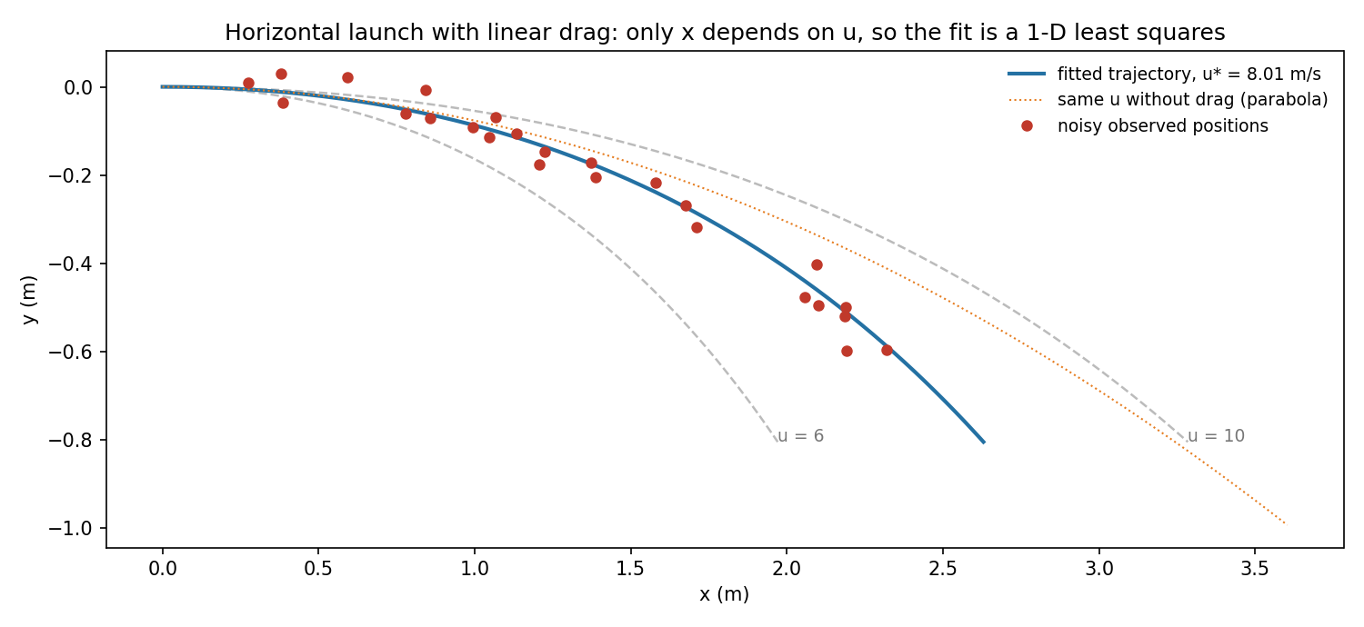
Sanity checks: for small $t$, $e^{-kt} \approx 1 - kt + k^2t^2/2$ gives $x \approx ut$ and $y \approx -\frac12 g t^2$, the drag-free parabola; for large $t$ the ball stops moving forward at $x_\infty = mu/b$ and falls at the terminal speed. (These formulas match a numerical ODE solution to $10^{-7}$ m.)

(b) Best launch speed. Only $x$ depends on $u$, and it does so linearly: $x(t;u) = u\,\varphi(t)$ with $\varphi(t) = \frac{m}{b}(1 - e^{-bt/m})$. The $y$ terms of $L(u)$ are constants. So we have a one-parameter least-squares regression through the origin:

$$\frac{dL}{du} = -2\sum_i \varphi(t_i)\big(\hat x_i - u\,\varphi(t_i)\big) = 0 \;\Longrightarrow\; u^\ast = \frac{\sum_{i=1}^n \hat x_i\,\varphi(t_i)}{\sum_{i=1}^n \varphi(t_i)^2} = \frac{b}{m}\cdot\frac{\sum_i \hat x_i\,(1 - e^{-bt_i/m})}{\sum_i (1 - e^{-bt_i/m})^2} .$$

$L$ is a convex parabola in $u$, so this is the global minimum. On simulated noisy data with true $u = 8$ m/s it returns $u^\ast = 8.01$.

A3. Two metrics hidden in code

(a) The string metric is the Jaro similarity. Two characters match if they are equal and their positions differ by at most $\lfloor \max(|s_1|,|s_2|)/2\rfloor - 1$; each character is used at most once. Let $m$ be the number of matches and $t$ the number of matched characters that are in a different order in the two strings (the second loop compares the matched characters in order). Then

$$\mathrm{Jaro}(s_1, s_2) = \begin{cases} 1 & s_1 = s_2 \\ 0 & m = 0 \\ \dfrac13\left(\dfrac{m}{|s_1|} + \dfrac{m}{|s_2|} + \dfrac{m - t/2}{m}\right) & \text{otherwise} \end{cases}$$

where $t/2$ is the number of transpositions.

(b) Where it beats exact match. Matching people's names in records: deduplicating patient or student databases, or searching a directory despite typos ("Shah" vs "Sah", "Aryan" vs "Aryna"). Exact match fails on any typo or transposition; Jaro gives a graded similarity that is tolerant to small, local errors and is designed for short strings.

(c) The search metric is Okapi BM25.

$$\mathrm{score}(q, d) = \sum_{t \in q,\; n_t > 0} \ln\!\left(\frac{N - n_t + 0.5}{n_t + 0.5} + 1\right)\cdot \frac{n_{t,d}\,(k + 1)}{n_{t,d} + k\left(1 - b + b\,\dfrac{L_d}{L_{\text{avg}}}\right)}$$

(the sum runs over the query's term list, so a repeated query term counts each time). The first factor is an IDF: rare terms weigh more. The second is a term frequency that saturates: it grows with $n_{t,d}$ but never exceeds $k + 1$.

(d) The role of $b$. It sets how much the document length normalises the term frequency. With $b = 1$, a document twice as long as average needs twice as many occurrences to get the same credit. With $b = 0$ the length factor disappears: there is no length normalisation, $n_{t,d}$ is compared with the constant $k$, and long documents are favoured simply because they contain more occurrences of everything. Typical values are $b \approx 0.75$.

A4. Debugging the motif scanner

Bugs and inefficiencies in the code (each was confirmed by running the code against a brute-force implementation of the specification):

lines	issue	fix
26	When the T of GAT is read, start = i overwrites the position of the G with that of the T, so every reported position is off by 2 (GATTAC returns [2] instead of [0]).	Delete start = i (keep the position set at the G).
11-12	Every N is skipped, including inside the patterns, so GNAT or TNAC are accepted although the specification forbids an N inside GAT or TAC (GNATCCTAC wrongly returns a match).	if base == 'N': reset partial matches first: if phase in (1, 2): phase = 0 and elif phase in (4, 5): phase = 3, then continue.
33-34	sequence[:i].count('N') rescans the whole prefix at every character: $O(n^2)$ time. It is also wrong: Ns are already never counted in gap (they hit continue), and subtracting all Ns since the start of the sequence (even those before the GAT) widens the window.	if gap > K: (no N counting at all).
32-36	Off-by-one in the window: gap is incremented before testing whether the base is the T of TAC, so the T itself is counted as a separating base. A TAC exactly $K$ bases away is rejected (GAT + 10 A + TAC returns nothing).	Test for T first and count the base only if it is not the start of TAC: if base == 'T': phase = 4 else: gap += 1; if gap > K: phase = 0.
29, 41, 48	Failed partial matches do not restart properly. In phase 2 a G should start a new GAT (GAGATCCTAC misses the GAT at 2). In phases 4 and 5 a T can itself be the start of TAC (GATCCTTAC and GATTATAC are missed).	Phase 2: elif base == 'G': phase = 1; start = i. Phases 4 and 5: if base == 'T': phase = 4.
46 and the design	After a match, phase = 0 throws away the current GAT, and while waiting for a TAC the machine ignores new GATs: overlapping motifs (GATCGATCCTAC should give [0, 4]) are lost, although the specification asks for all GAT-TAC pairs within the window.	A single state variable cannot track several open GATs. Keep a list of open GAT positions, or better, use the two-pass design below.

A clean linear-time replacement records the GAT and TAC positions, plus a running count of non-N bases, then pairs them:

def find_motifs(sequence):
    non_n = [0]                                   # non_n[i] = number of non-N bases in sequence[:i]
    for ch in sequence: non_n.append(non_n[-1] + (ch != 'N'))
    gats = [i for i in range(len(sequence) - 2) if sequence[i:i+3] == "GAT"]
    tacs = [j for j in range(len(sequence) - 2) if sequence[j:j+3] == "TAC"]
    results, lo = [], 0
    for i in gats:                                # both lists are sorted: two pointers
        while lo < len(tacs) and tacs[lo] < i + 3: lo += 1
        j = lo
        while j < len(tacs) and non_n[tacs[j]] - non_n[i + 3] <= K:
            results.append(i); j += 1             # one entry per valid (GAT, TAC) pair
    return results

Searching for the literal strings "GAT" and "TAC" automatically forbids an N inside a pattern, the prefix count makes every gap an $O(1)$ subtraction, and the output equals the brute-force reference on 20 000 random sequences.

A5. Dashboards for a live speech

(a) Whom to answer. A live scatter plot with one point per comment. The x-axis is the sentiment score from $-1$ to $+1$, with a vertical line at 0. The y-axis is the author's follower count on a log scale, because follower counts span many orders of magnitude. Colour is a diverging scale (red for negative, green for positive), marker shape shows the channel, and older points fade out so that only the last few minutes stay visible. The top-left region (very negative, many followers) is the "rebut first" zone, the top-right the "amplify first" zone. Hovering shows the text, and a side table lists the top 10 of each zone, sorted by followers times |sentiment|.

(b) When and where sentiment spikes. A multi-line time-series chart, or small multiples with one panel per channel. The x-axis is the speech time (0 to 120 minutes), the y-axis the rolling mean sentiment over, say, one-minute windows, with one coloured line per channel and a shaded band for the standard error (thin when there are many comments). Underneath, on a shared time axis, bars show the comment volume per minute, so that a spike based on three comments is not over-interpreted. Mark spikes automatically, for example where the change between consecutive windows exceeds 3 standard deviations, with vertical markers labelled by channel, and annotate the speech segments (topics) along the time axis. A channel-by-time heatmap of the sentiment change is a compact alternative.

Section B: Introductory ML Theory

B1. Product quality tiers

(a) The decision tree. In the plot, the tier depends on the category and on the region in a way that differs from one category to another. For Clothing (squares), Premium sits in the middle of the plane, Standard in two separate corners (low rating with many reviews, and high rating with few reviews), and Counterfeit at low ratings and in a high-rating, high-volume patch. For Electronics (circles), Counterfeit appears both at low ratings and in a top-right cluster with very high ratings and many reviews (plausibly fake reviews). Books (triangles) have their own layout. So each class is multimodal and the boundaries are category-specific and roughly axis-aligned.

• A decision tree can split on the category first and then on rating and review-count thresholds, carving out exactly such rectangles. It captures interactions and multimodal classes without any feature engineering.
• Naive Bayes models each numeric feature, for each class, by a single Gaussian and assumes the features independent given the class. A class living in two distant patches gets one wide Gaussian centred between them (where it may have no points), and the category cannot change how the numeric features behave.
• Logistic regression draws linear boundaries in (rating, log count). One-hot category features only shift the intercept of each class score, so all categories share the same slopes, and multimodal classes cannot be represented at all.

(b) Naive Bayes: 24 parameters (20 free). It has 3 class priors (2 free, since they sum to 1). For each class and each numeric feature it learns a mean and a variance: $3 \times 2 \times 2 = 12$. For each class it learns a categorical distribution over the 3 categories: $3 \times 3 = 9$ (6 free). In total $3 + 12 + 9 = 24$, or $2 + 12 + 6 = 20$ free parameters.

(c) Multinomial logistic regression: 18 parameters (10 identifiable). The inputs are rating, log count and 3 one-hot columns: 5 weights plus a bias for each of the 3 classes, $3 \times 6 = 18$. Two redundancies remain: the three one-hot columns sum to 1 and are collinear with the bias (drop one column), and softmax is unchanged if the same vector is added to all classes (fix a reference class). The identifiable count is therefore $2 \times (1 + 2 + 2) = 10$, i.e. 15 if you only drop one one-hot column.

(d) Feature engineering for LR. Add interactions between category and the numeric features (rating x category, log count x category), so that each category gets its own slopes, together with non-linear terms that can represent several patches: binned rating and review count (one-hot bins) and their products, or polynomial terms up to degree 2 or 3. Category-specific bins essentially reproduce the tree's rectangles inside a linear model.

B2. Predicting days to readmission

(a) Two feature-engineering steps.

1. An interaction term age_years x num_prior_admissions (or prior admissions within age bands). The residuals show that the effect of prior admissions depends on age: with many prior admissions, elderly patients come back later than the model predicts and young patients sooner. An additive model forces one common slope for prior admissions; the product lets that slope grow with age.
2. A piecewise representation of age: hinge features $\max(0, \text{age} - 40)$ and $\max(0, \text{age} - 70)$ (a linear spline with knots at 40 and 70), or age bands 18-40, 40-70, 70+. The model can then be flat, then gently rising, then steep, as the residual plot shows, while staying linear in its parameters.

(b) Lasso. One-hot coding the 200 diagnosis codes, plus 50 sparse flags, plus the new interaction and spline features, gives hundreds of sparse columns. Most diagnosis codes are rare and probably irrelevant. Lasso's $\ell_1$ penalty sets most of these coefficients exactly to zero, which selects features, reduces variance on rare categories and keeps the model interpretable for clinicians. Plain linear regression has no regularisation, so it overfits and gives unstable coefficients for rare codes. Ridge shrinks every coefficient but keeps them all, so it neither selects nor gives a sparse, readable model. (Elastic net is a good compromise if groups of codes are correlated.)

(c) Mean absolute error. The few patients readmitted after more than 180 days because of palliative care are outliers relative to the population of interest. MSE squares their residuals, so they dominate the loss and drag the fitted model towards them. MAE grows linearly, so it is robust; it targets the conditional median, a better "typical delay" in a skewed distribution. (Even better: flag or model the palliative-care discharges separately, since they come from a different process.)

B3. Clustering 300 000 contracts

(a) Spherical k-means with cosine similarity.

• Standard k-means on binary bag-of-words vectors measures Euclidean distance, which is dominated by document length: long contracts contain many terms and are far from everything, so clusters form by length rather than by topic, and the centroids become dense 30 000-dimensional vectors.
• Agglomerative clustering needs pairwise similarities: $300\,000^2/2 \approx 4.5 \times 10^{10}$ pairs, which is infeasible in time and memory.
• DBSCAN relies on a density radius, which is ill-defined in 30 000 sparse dimensions (distances concentrate). It does not let you ask for 8 clusters and labels many documents as noise.
• Spherical k-means normalises each document to unit length, so cosine similarity compares which terms appear, not how many; this is the standard similarity for text. Each iteration costs $O(\text{non-zeros} \times k)$, linear in the corpus, and $k = 8$ is set directly.

(b) When clustering then labelling (B) beats a classifier (A). B wins under the cluster assumption: the 8 contract types form compact, well-separated clusters in this representation (each cluster is nearly pure), and the labelled documents are spread over all clusters. Then B exploits the 299 500 unlabelled documents, while A must learn a 30 000-dimensional classifier from only 500 examples, about 60 per class, and overfits. When the assumption fails (types split over several clusters, or several types merged into one), majority labels propagate errors to entire clusters. More robust variants:

• over-cluster (e.g. $k = 50$ to 100) so that each small cluster is purer, then label clusters by majority, leaving clusters without labels for review;
• seed the clustering with the labelled documents (seeded or constrained k-means);
• use semi-supervised learning: train the classifier of A, then add pseudo-labels from high-purity clusters or high-confidence predictions (self-training, label propagation);
• assign a cluster label only when its labelled members agree strongly, and fall back to the classifier otherwise.

B4. Practical modelling aspects

(a) Two models. Model A (63 % train, 61 % validation) underfits, i.e. has high bias: train and validation scores are both low and close. Increase capacity or information: a more expressive model, better features, less regularisation, longer training. Model B (97 % / 68 %) overfits, i.e. has high variance, with a 29-point gap. Regularise (weight decay, dropout, smaller depth), stop early, collect more data or augment it, or ensemble. The target is the best validation score, not the best training score.

(b) Two splits. (The statement announces three strategies but lists two.)

• Random split measures how well the model fills in randomly missing entries of the user-movie matrix for known users and movies. It is misleading because it leaks the future: the model trains on ratings made after the test ratings (later tastes, a movie's eventual popularity). It also never tests cold start (new users or new movies), so it overestimates deployed performance.
• Time split measures what we want in production: predicting future ratings from the past. It can be misleading in other ways: the test period contains new users and movies with no history (cold start), and seasonal or popularity trends make one particular period unrepresentative; heavy users also dominate the most recent ratings. A rolling time-based evaluation, with cold-start users reported separately, gives a fairer picture.

(c) MSE versus MAPE. MSE weighs absolute errors, squared: an error of 10 units costs the same on an item that sells 1000 units as on one that sells 10. MAPE weighs relative errors, $|\hat y - y|/|y|$, so low-volume items dominate it. The two optima also differ: MSE is minimised by the conditional mean, while MAPE is minimised by a weighted median with weights $1/|y|$, which sits lower. A model can therefore be excellent in MSE (getting the big sellers right) and poor in MAPE. Fixes, any of which works: train with sample weights $w_i = 1/|y_i|$ on an absolute-error loss, which is exactly MAPE; train on $\log y$ (log errors approximate relative errors); or use MAPE as a custom loss in gradient boosting. In every case, choose hyperparameters and models on validation MAPE.

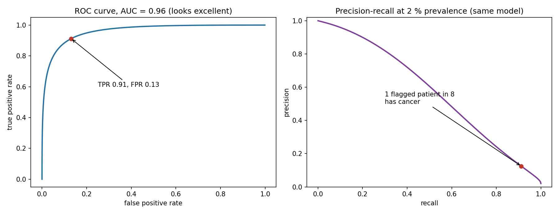
(d) High AUC, low precision. AUC is the probability that a random positive gets a higher score than a random negative. It is computed from TPR and FPR, so it ignores prevalence and does not depend on any threshold. With 2 % positives there are 49 negatives per positive, so even a small FPR produces many false alarms: with $\text{TPR} = 0.91$ and $\text{FPR} = 0.13$, a point that lies on an AUC 0.96 curve, precision is $\frac{0.02 \times 0.91}{0.02 \times 0.91 + 0.98 \times 0.13} \approx \frac18$, exactly what the clinician saw. The team should have examined the precision-recall curve and its area (average precision), and the precision and recall at the operating threshold, chosen deliberately rather than left at 0.5.

Section C: ML Applications

C1. Visual math problem solver

(a) Tasks. Parsing a document layout, which separates the text from the graph image. Chart understanding: detecting the axes, ticks and labelled points, and recovering the curve's coordinates. Question understanding, i.e. semantic parsing of the text into a structured goal. Symbolic reasoning: fitting the cubic through the read points and solving for the requested quantity. Text generation: writing a step-by-step explanation. A vision-language model can merge several of these steps, but it must be checked by a computation.

(b) Data. Generate it synthetically. Sample random polynomials, conics and lines with random labelled points, render them with matplotlib under varied styles (grids, fonts, ranges, noise), render questions from templates and paraphrase them with an LLM. The ground truth (exact coefficients, answers and solutions) comes for free. Add a smaller set of real textbook and exam pages, annotated by teachers, for evaluation and fine-tuning, and step-by-step solutions written by tutors for the explanation style.

(c) Pipeline.

1. PDF parsing: the PDF goes in; the question text (extracted directly, no OCR needed since it is digital) and the raster image of the graph come out.
2. Graph parsing: the image goes in; detection of axes and ticks (object detection), OCR of the tick labels, a pixel-to-coordinate mapping (a linear fit from tick positions to values), segmentation of the curve, and detection and OCR of the labelled points. Out: a list of (x, y) coordinates of the labelled points and sampled curve points.
3. Question parsing: the text goes in; classification of the problem type and extraction of the target (here the "leading coefficient") with an LLM or a template parser. Out: a structured query.
4. Solving: points plus query go in; least-squares fitting of the right function family (a cubic) using the exact labelled points first, then a symbolic solve with SymPy. Out: the answer and the intermediate quantities.
5. Explanation: the structured steps go in; an LLM writes the step-by-step solution from the verified intermediate results, without being allowed to invent numbers. Out: the solution text and the final answer.
6. Confidence check: if the fit residual is large or the parsed points are inconsistent, flag the problem for human review.

(d) Metrics. Final-answer accuracy (exact match, or relative error below a tolerance for numerical answers). Graph-parsing accuracy: the error of the extracted point coordinates, and the curve-recovery error such as RMSE between true and recovered curves. Step correctness, judged by teachers or by automatic checking of each intermediate quantity. Latency per problem.

C2. Indian Sign Language interpreter

(a) Tasks and challenges. Voice to ISL is speech recognition (ASR), then translation from English text to ISL gloss sequences (sequence-to-sequence), then sign-sequence generation for the avatar (gesture synthesis, motion generation). ISL to voice is continuous sign language recognition from video (pose and hand tracking plus spatio-temporal sequence modelling), translation from gloss to English, then speech synthesis (TTS). Challenges that would not exist with word-for-word correspondence: in Voice to ISL, the word order and grammar must be re-ordered (ISL tends towards subject-object-verb order and drops function words such as articles), and grammatical information must be encoded through facial expressions and spatial placement, not extra signs. In ISL to Voice, one sign carries meaning simultaneously through hand shape, movement and face (questions and negation are often marked by facial expression), so recognition is not a sequence of isolated "word" signs, and the English output must add words, such as articles and tense, that are not signed.

(b) Data. Voice to ISL needs English speech (Indian accents, counter vocabulary) for ASR, if not pretrained, then a parallel corpus of English sentences and ISL gloss sequences, then a motion-capture or pose dataset of signers for each sign and its non-manual markers to drive the avatar. ISL to Voice needs videos of continuous ISL sentences from many signers (varied skin tones, clothing, lighting and camera angles, left- and right-handed), annotated with glosses and English translations, plus isolated-sign datasets for pretraining. Domain-specific phrases for government counters (forms, documents, payments) are a priority in both directions. Deaf signers must be involved in collecting and validating the data.

(c) Pipelines.

• Voice to ISL: audio, then voice activity detection and ASR (Whisper-like), giving English text; then text normalisation and simplification; then translation to an ISL gloss sequence with non-manual markers (a transformer seq2seq or an LLM fine-tuned on the parallel corpus); then mapping glosses to motion clips or generating pose sequences, with smooth transitions (co-articulation) and facial expressions; finally rendering of the avatar in real time.
• ISL to Voice: camera frames go through pose estimation (MediaPipe or OpenPose keypoints for hands, body and face), giving keypoint time series. A spatio-temporal model (a transformer or a temporal CNN over keypoints, trained with CTC loss) does continuous recognition and outputs a gloss sequence. A seq2seq model translates glosses into a fluent English sentence, which can also be done end to end from video to text, and TTS produces audio. A confidence score is shown on screen, with a "please repeat" fallback when it is low.

(d) Metrics. For Voice to ISL: ASR word error rate, BLEU or chrF of the generated gloss against reference glosses, and human comprehension by deaf users (the percentage of avatar sentences understood correctly), plus naturalness ratings. For ISL to Voice: word error rate of the recognised glosses, BLEU or chrF of the English translation, and task-success rate in counter scenarios. Real time, for both: end-to-end latency (from the end of the utterance or signing to output) at the 50th and 95th percentiles, with a target such as under 1 to 2 seconds, and throughput in frames per second on the counter's hardware. Report accuracy at the latency budget, not offline accuracy.

C3. Medical symptom triage

(a) Tasks. Multimodal four-class classification (free text plus structured questionnaire), which is ordinal (Emergency > Urgent > Routine > Self-care) and imbalanced, with noisy labels from disagreeing doctors. It also involves extracting clinical concepts from the text (symptoms, duration, severity, red flags), calibrated uncertainty estimation, and selective prediction (deferring to a human).

(b) Data. Historical helpline and emergency-department records linking the patient's description and answers to the triage decision and to the eventual outcome (admission, ICU, diagnosis), which is a less noisy target than a single doctor's label. Collect multiple doctor labels for each case, at least for the training subset and the whole test set, to estimate disagreement and use soft labels; an expert-adjudicated test set; oversampled rare emergencies; and coverage of languages, ages and demographics for fairness checks. Prospective shadow-mode data (the model runs silently next to nurses) for the final evaluation.

(c) Pipeline.

1. Input check and red-flag rules: text and answers go in; deterministic rules (chest pain with shortness of breath, stroke signs, suicidal ideation) send the case directly to Emergency. Safety must not depend on the model.
2. Text encoding: the free text goes in; a clinical language model (e.g. BioBERT) or LLM extraction gives an embedding and structured symptom features.
3. Fusion and classification: text features plus questionnaire features go in; a classifier (gradient boosting, or a neural head) trained with an ordinal, cost-sensitive loss and soft labels from the doctors' disagreement outputs calibrated probabilities over the 4 levels.
4. Decision: probabilities go in; a cost-sensitive decision rule (expected cost under an asymmetric cost matrix, where under-triage is far costlier) outputs a level, and if confidence is low or the case is borderline, the case is escalated to a human nurse or doctor.
5. Output: the level plus an explanation (the key symptoms) for the human reviewer, and logging for monitoring.

(d) Metrics. Accuracy is insufficient because serious cases are rare: predicting "Routine" for everyone can be very accurate while missing every emergency, and accuracy treats all errors alike, although under-triaging an emergency is far worse than over-triaging. Use instead: sensitivity (recall) for Emergency and for Urgent, with a high target such as at least 98 % for Emergency; the under-triage and over-triage rates; a cost-weighted error with the clinical cost matrix; quadratic weighted kappa for ordinal agreement, compared with doctor-doctor agreement (which is the ceiling); calibration error; and the escalation rate, i.e. the human workload.

C4. Electricity demand forecasting

(a) Tasks and what is special. Multi-step, multi-series time-series regression (24 hourly values per zone), ideally probabilistic (quantiles), plus change-point or drift detection. Unlike independent examples, the observations are temporally dependent (autocorrelated, with daily, weekly and yearly seasonality) and non-stationary (gradual seasonal drift and permanent structural breaks). Random shuffling and K-fold cross-validation would leak the future into training.

(b) Extra data. Weather forecasts and history (temperature, humidity, solar radiation, wind, since temperature drives heating and cooling); the calendar (hour, day of week, public holidays, festivals, school terms); special events; economic and industrial activity per zone (new factories, planned connections, shift schedules), which signal structural breaks in advance; electricity prices and tariffs; rooftop solar capacity (behind-the-meter generation reduces measured demand); and grid outages and maintenance logs to clean the history.

(c) Pipeline.

1. Ingestion and cleaning: raw meter readings per zone go in; anomaly detection removes outages and meter faults, and gaps are imputed. Out: clean hourly series.
2. Change-point detection: the series go in; statistical tests (CUSUM, Bayesian change points) or business events flag permanent level shifts. Out: regime boundaries, so that training data before a break can be down-weighted or adjusted.
3. Feature construction: series, weather forecasts and calendar go in; lags (24 h, 168 h), rolling statistics, calendar encodings, forecast weather and zone identifiers come out.
4. Forecasting model: the features go in; a global gradient-boosting model or a neural forecaster (temporal convolution, transformer) trained across zones outputs the next 24 hourly values per zone. Train it with a quantile (pinball) loss at a high quantile (e.g. 0.9) or an asymmetric loss, since under-forecasting is costlier.
5. Online adaptation: recent errors go in; retraining on a sliding window or with recency weights, plus monitoring for drift, keep the model up to date.
6. Reconciliation and decision: zone forecasts are made consistent with the city total (hierarchical reconciliation), and the chosen quantile is sent to grid planning.

(d) Metrics. Evaluate with rolling-origin backtests (train on the past, forecast the next 24 h, move forward), never random splits. Use MAPE or MAE per zone and horizon for overall accuracy, and an asymmetric cost that matches the business: the pinball loss at the chosen quantile, or a weighted error such as $c_u \max(0, y - \hat y) + c_o \max(0, \hat y - y)$ with $c_u > c_o$. Track the under-forecast rate and peak-hour error, since shortfalls at the daily peak are the expensive ones, and coverage of the prediction intervals. Report performance separately after structural events to check how fast the model adapts.

What to remember

• Look for structure before computing: $u^\top A^\top A u - 2u^\top A^\top A v + v^\top A^\top A v$ is a squared norm, and a model that is linear in a parameter turns its fit into one-line least squares.
• Recognise classic metrics from their code: Jaro (matching window, transpositions), BM25 (IDF times saturated, length-normalised term frequency), and know what each knob does.
• Debug against the specification, not the code: write a brute-force reference, generate random and edge-case inputs (patterns next to each other, N inside patterns, gaps of exactly $K$), and compare.
• Choose models from the geometry of the data: multimodal, category-specific regions favour trees; linear models need interactions and bins; sparse high-dimensional text favours cosine similarity and $\ell_1$ regularisation.
• Evaluation must mirror deployment: time-based splits for time-dependent data, precision and PR curves under rare positives, the loss that matches the business metric (MAPE, asymmetric costs), and a human in the loop when the model is unsure.