Theory (Part 1)

The problem in brief

This is the written part of the INAIO 2025 final stage: 65 points of short questions in three sections. Section A (Foundations, 30 points) checks that you can read and write the everyday code of ML (pandas merges, batched tensor algebra, plots of high-dimensional data, ranking metrics, cross-validation) and do the calculus behind it. Section B (ML Theory, 20 points) asks for modelling judgement: which classifier suits a data shape, how to pick an operating point on a ROC curve, which output layer goes with which loss, LoRA and vision architecture choices. Section C (Applications, 15 points) gives three real-world systems to design from scratch.

The answers below are our own. Every numerical answer was checked in Python (the checks are in the solution code): the pandas output was executed, the attention code was run on random tensors, the closed-form gradients were compared with finite differences and the ROC operating points were computed from points read off the figure.

How you are scored

Points are written next to each question (typically 0.5 to 2 points per sub-question), and the organisers state that answers are read with "the most generous interpretation". Code does not need to run, but must use the right functions and logic; maths may be given in words, plain text or LaTeX. Some questions carry unspecified bonus points. There is no pass mark in the statement, so the target is simply a full, justified answer to every sub-question.

Section A: Foundations

A1. Merges and group-by

1. The output. Step by step:

• The left merge keeps all four customers. Customers 1 and 2 have two orders each; customers 3 and 4 have none, so they appear once with NaN in order_id, product_id, amount. Order 104 (customer 5, unknown) is dropped: a left join keeps only keys of the left table. Because of the NaNs, amount and product_id become floats.
• The inner merge on product_id keeps only rows whose product exists in both tables. The two NaN rows of customers 3 and 4 have no match and disappear. The 4 remaining orders (101, 102, 103, 105) use products 11 and 12, both known.
• Group by (country, category): US/A = order 101 (250), US/B = order 105 (200), UK/A = order 103 (300), UK/B = order 102 (100).

  country category  total_amount  order_count
0      UK        A         300.0            1
1      UK        B         100.0            1
2      US        A         250.0            1
3      US        B         200.0            1

Groups come out sorted by key (UK before US). Germany never appears and fillna(0) does nothing, because a group-by only creates groups that exist in the data: it never invents a (DE, A) row with zeros.

2. What was dropped and why. Order 104 is lost in the first merge (its customer 5 is not in the customer table, and a left join keeps only left keys). Customers 3 (US) and 4 (DE) survive the left join with empty orders but are removed by the inner join, because NaN matches no product. Product 14 (category C) is never ordered, so category C never appears. If the goal is a report that shows zero-sales countries, the second merge should also be a left join and the counts should be computed on order_id (which count skips when it is NaN).

A2. Scaled attention in PyTorch

K_scaled = K * s                                   # (B, Nk, D): s (D,) broadcasts over the last axis
S = Q @ K_scaled.transpose(-2, -1)                 # (B, Nq, D) @ (B, D, Nk) -> (B, Nq, Nk)
A = torch.softmax(S, dim=-1)                       # (B, Nq, Nk): normalised over the keys
C = A @ V                                          # (B, Nq, Nk) @ (B, Nk, Dv) -> (B, Nq, Dv)

with $B$ = batch size, $N_q$ = number of queries, $N_k$ = number of keys, $D$ = embedding dimension, $D_v$ = value dimension. The two subtle points are broadcasting (s has shape (D,) and aligns with the last axis of K automatically) and transposing only the last two axes, not the batch axis. The same thing in one line: torch.einsum('bqd,d,bkd->bqk', Q, s, K).softmax(-1) @ V. (Equivalently one may scale Q instead of K: $Q\,\mathrm{diag}(s)\,K^\top$ is the same matrix.)

A3. Visualising 10 000 digit images

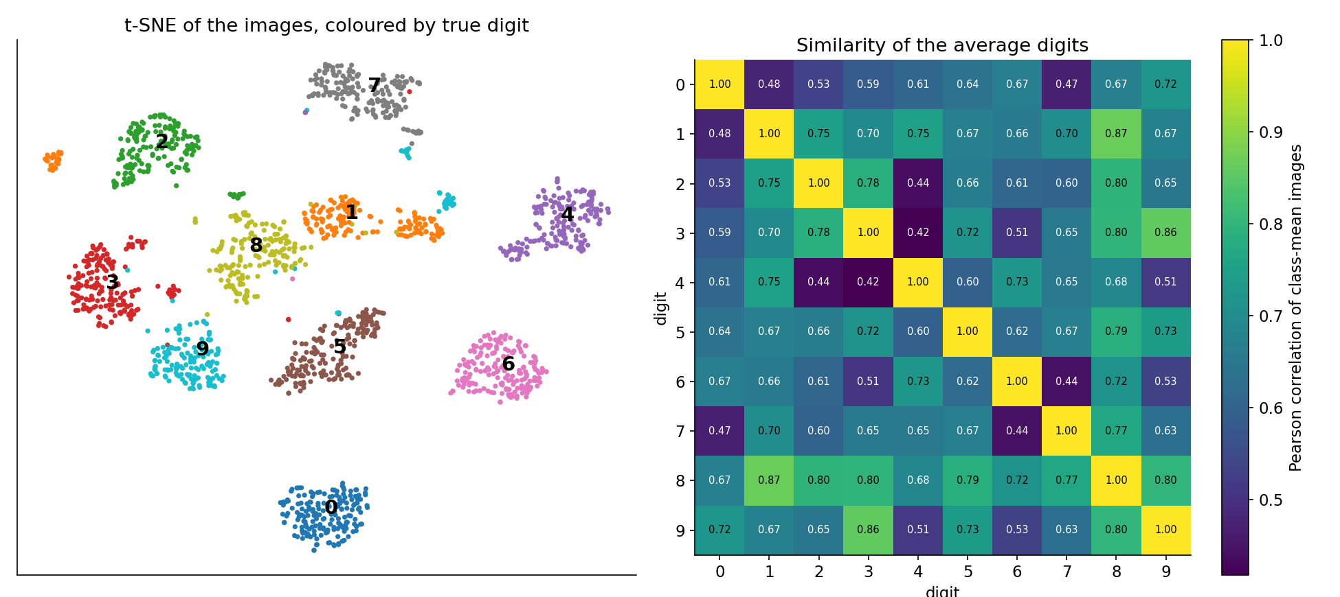
1(a) Strategy. 784 dimensions cannot be plotted, so project to 2-D and colour each point by its label. A linear projection (PCA) is quick but keeps only global variance and usually leaves digit classes overlapping. A non-linear neighbour-preserving embedding (t-SNE or UMAP) is the right tool: it is designed to keep points that are close in the 784-D space close in the plane, which is precisely the question "do same-digit images form clusters?". Standard practice: PCA to about 50 dimensions first (removes noise and makes t-SNE fast), then t-SNE. Caveat to state: in t-SNE, distances between clusters and cluster sizes are not meaningful, only neighbourhoods.

1(b) Code.

from sklearn.decomposition import PCA
from sklearn.manifold import TSNE
import matplotlib.pyplot as plt
Z = TSNE(n_components=2, perplexity=30, init="pca", random_state=0) \
        .fit_transform(PCA(n_components=50).fit_transform(X / 255.0))
plt.figure(figsize=(8, 8))
sc = plt.scatter(Z[:, 0], Z[:, 1], c=y, cmap="tab10", s=3)
plt.legend(*sc.legend_elements(), title="digit")
plt.title("t-SNE of MNIST digits"); plt.show()

2(a) Class similarity. Compute the mean image of each class (average of its 1 000 or so vectors), then the $10\times 10$ matrix of Pearson correlations (or cosine similarities) between these 10 mean vectors, and show it as an annotated heatmap. High off-diagonal values flag pairs of digits that look alike on average (e.g. 3/5/8, 4/9, 7/9) and are therefore likely confusions for a classifier. It is also worth displaying the 10 mean images themselves.

2(b) Code.

import numpy as np, seaborn as sns
means = np.stack([X[y == d].mean(axis=0) for d in range(10)])   # (10, 784)
C = np.corrcoef(means)                                          # (10, 10)
sns.heatmap(C, annot=True, fmt=".2f", cmap="viridis",
            xticklabels=range(10), yticklabels=range(10))
plt.title("Correlation between class-mean images"); plt.show()

We ran both on scikit-learn's small 8x8 digits dataset (MNIST was not provided): the clusters separate cleanly and the most similar pairs of average digits are 1/8, 3/9 and 8/9.

A4. Reverse-engineering two ranking metrics

In both functions y is a list of relevance scores in the order the system ranked the items, and k is a cutoff.

Metric 1 (a): Average Precision at $k$. Let $\mathrm{rel}_i = 1$ if $y_i > 0$ and $0$ otherwise, $R = \sum_i \mathrm{rel}_i$ the total number of relevant items in the whole list, and $P@i = \frac{1}{i}\sum_{j\le i} \mathrm{rel}_j$ the precision of the top $i$. The variable p counts relevant items seen so far, so p/idx is exactly $P@i$ at each relevant position:

$$\mathrm{AP@}k = \frac{1}{\min(R, k)} \sum_{i=1}^{k} \mathrm{rel}_i \cdot P@i$$

(and $0$ if there is no relevant item in the top $k$). Example: $y = (1,0,1,0,0,1)$, $k=3$: $(1/1 + 2/3)/\min(3,3) = 0.556$.

(b) Use and meaning. Search engines, recommendation, retrieval for RAG, object-detection mAP: any task with binary relevance where you care about where the relevant items are placed. AP rewards putting relevant items early; averaged over queries it gives MAP@k.

(c) Why $\min(R,k)$. It is the largest number of relevant items that can appear in the top $k$. Dividing by it makes a perfect ranking score exactly 1 even when $R > k$ (dividing by $R$ would penalise the system for relevant items it was not allowed to show) and when $R < k$.

Metric 2 (a): NDCG at $k$. With graded relevances $y_i$,

$$\mathrm{DCG@}k = \sum_{i=1}^{k} \frac{2^{y_i} - 1}{\log_2(i + 1)}, \qquad \mathrm{NDCG@}k = \frac{\mathrm{DCG@}k(\text{system order})}{\mathrm{DCG@}k(\text{ideal order: } y \text{ sorted decreasingly})}$$

(the code's log2(i + 2) with $i$ starting at 0 is $\log_2(\text{rank} + 1)$), and 0 if the ideal DCG is 0.

(b) Use and meaning. Ranking with graded relevance (web search with "perfect / good / fair" labels, product search, recommendation). The gain $2^{y}-1$ makes highly relevant items count much more; normalising by the ideal DCG gives a score in $[0,1]$ comparable across queries with different numbers of relevant items.

(c) The log term is a position discount: an item at rank $r$ is worth $1/\log_2(r+1)$ of its gain, modelling the fact that users look at the top results much more than the lower ones (rank 1 counts fully, rank 3 counts half, rank 7 a third). The discount decreases slowly, so lower ranks still matter a little.

A5. Cancer screening: what is wrong with the tuning code

1. Problems.

1. Accuracy is the wrong selection metric. With 1 % positives, "always benign" scores 99 % accuracy; grid search will happily pick the model that misses most cancers. The clinical goal (few missed cancers, few needless biopsies) is about recall and precision on the positive class.
2. Plain KFold on a 1 % class. Folds get very different and sometimes tiny numbers of positives, so validation scores are noisy and some folds may have almost no positive at all.
3. No handling of class imbalance in training (no class weights, no resampling): the forest learns to predict "benign".
4. Prior shift is ignored. The test population has 5 % positives, not 1 %. With identical class-conditional distributions, the model's probabilities are miscalibrated for the hospital: they underestimate the risk. Any threshold chosen on the training prior is wrong at the hospital.
5. The default 0.5 threshold of predict is never chosen from the clinical costs, and the test is again summarised by accuracy, which at 5 % prevalence says almost nothing (95 % for the trivial model).
6. Minor: random_state only on the forest, no held-out validation for the threshold, and no report of recall, precision or a confusion matrix.

2. Fixes.

1. Use StratifiedKFold(n_splits=5, shuffle=True, random_state=0).
2. Select hyperparameters with an imbalance-aware score: scoring='average_precision' (area under the precision-recall curve) or ROC-AUC, or an $F_\beta$ with $\beta > 1$ (e.g. $F_2$) to weight recall more.
3. Use class_weight='balanced' (or 'balanced_subsample'), or resample the training data.
4. Correct for the prior shift. By Bayes, if only the priors change, the posterior odds are multiplied by the ratio of prior odds:

$$\frac{p_{\text{test}}}{1-p_{\text{test}}} = \frac{p_{\text{train}}}{1-p_{\text{train}}}\cdot\frac{0.05/0.95}{0.01/0.99} \approx 5.2\,\frac{p_{\text{train}}}{1-p_{\text{train}}} .$$

(If class weights were used, replace the training prior by the effective one, 50 %.) Calibrate the probabilities first (CalibratedClassifierCV), then apply this adjustment. 5. Choose the threshold deliberately, on validation data with the adjusted probabilities: e.g. the highest threshold that keeps recall $\ge 95$ %, then check the precision (biopsies per cancer found). Report recall, precision, the confusion matrix and PR-AUC on the test set, not accuracy.

A6. A systematic plan when the model falls short

intervention family	what tells you it is the right one
Reduce bias: bigger or more flexible model, better features, less regularisation, train longer	training error itself is too high (above the target); learning curves of train and validation are both high and close together
Reduce variance: more data, data augmentation, stronger regularisation (weight decay, dropout, smaller trees), early stopping, ensembling	low training error but large train/validation gap; validation curve over a complexity hyperparameter goes back up; validation error still falling as the training set grows (learning curve)
Fix the data: clean labels, remove leakage or duplicates, fix preprocessing, handle missing values	error analysis on the worst mistakes shows wrong labels or broken inputs; suspiciously high validation scores (leakage)
Handle imbalance and the metric: class weights, resampling, threshold tuning, metric aligned with the goal	confusion matrix and per-class recall show minority classes ignored; PR curve; calibration plot
Fix optimisation: learning rate, schedule, initialisation, normalisation, optimiser	training loss curve noisy, diverging or flat from the start; gradient norms exploding or vanishing
Different model family or architecture (inductive bias that matches the data: CNN for images, trees for tabular data)	residual plots or errors with structure the model cannot express; strong gap to a simple well-suited baseline
Distribution shift: re-weighting, domain adaptation, collecting data from the target domain	validation (same distribution as train) good but test or production bad; adversarial validation can distinguish train from test
Hyperparameter search (random or Bayesian, with proper CV)	validation score sensitive to hyperparameters; current values at the edge of the grid

The habit to show: first locate the error (bias, variance, data, metric, shift) with diagnostics, then choose the intervention; do not try interventions at random.

A7. Linear algebra and vector calculus

1. Projection onto the hyperplane $a^\top w = b$. The closest point lies along the normal $a$: $w_{\text{proj}} = w_{\text{new}} - t\,a$. Imposing $a^\top w_{\text{proj}} = b$ gives $t = (a^\top w_{\text{new}} - b)/\lVert a\rVert^2$:

$$w_{\text{proj}} = w_{\text{new}} - \frac{a^\top w_{\text{new}} - b}{\lVert a \rVert^2}\, a .$$

(It minimises $\lVert w - w_{\text{new}}\rVert^2$ under the constraint, as a Lagrange multiplier computation confirms: the gradient condition $2(w - w_{\text{new}}) = \mu a$ says the correction is parallel to $a$.) This is one step of projected gradient descent.

2. Gradient of $J(x) = x^\top B x + c^\top x$. Write $x^\top B x = \sum_{i,j} B_{ij} x_i x_j$; its derivative in $x_k$ is $\sum_j B_{kj}x_j + \sum_i B_{ik} x_i$. Hence

$$\nabla_x J = (B + B^\top)\,x + c ,$$

which reduces to $2Bx + c$ only when $B$ is symmetric. (Checked against finite differences for a random non-symmetric $B$.)

3. Jacobian of the softmax. With $p_i = e^{z_i}/\Sigma$, $\Sigma = \sum_j e^{z_j}$, the quotient rule gives $\partial p_i/\partial z_j = (\delta_{ij} e^{z_i}\Sigma - e^{z_i}e^{z_j})/\Sigma^2$:

$$J_{ij} = \frac{\partial p_i}{\partial z_j} = p_i(\delta_{ij} - p_j) \quad\Longleftrightarrow\quad J = \mathrm{diag}(p) - p\,p^\top .$$

Diagonal entries $p_i(1-p_i) > 0$, off-diagonal $-p_ip_j < 0$: raising one logit raises its own probability and lowers all others. Each row sums to 0 because the probabilities always sum to 1.

4. Minimiser of $L(x) = \sum_{i=1}^m (x-u_i)^\top M (x-u_i) + \lambda\lVert x\rVert^2$. A positive definite $M$ is taken symmetric (otherwise replace it by $(M+M^\top)/2$, which gives the same quadratic form). Then $\nabla L = 2\sum_i M(x - u_i) + 2\lambda x = 0$, so $(mM + \lambda I)\,x = M\sum_i u_i$:

$$x^\ast = (mM + \lambda I)^{-1} M \sum_{i=1}^{m} u_i = \big(M + \tfrac{\lambda}{m} I\big)^{-1} M\, \bar u , \qquad \bar u = \frac{1}{m}\sum_i u_i .$$

$mM + \lambda I$ is positive definite, so it is invertible and the Hessian $2(mM+\lambda I)$ confirms a unique minimum. Interpretation: the mean $\bar u$ shrunk towards 0; with $\lambda = 0$ we recover $x^\ast = \bar u$. (Checked against a numerical optimiser.)

Section B: ML Theory

B1. Matching the model to the data shape

Scenario 1: blobs, with the class decided by tissue type inside each blob. There are six compact clusters in the (AFP, bilirubin) plane, and inside each cluster two tissue types appear, each with its own class (e.g. top-left: circles are C, triangles are B; centre: circles are B, triangles are C). The class is an interaction between region and tissue type.

• (a) One-hot encode the tissue type, add a region feature (cluster id from k-means on standardised AFP and bilirubin, or RBF features centred on the clusters) and the products region x tissue. With these indicator features a linear classifier can separate everything.
• (b) Decision trees / random forests / gradient boosting: axis-aligned splits isolate a blob in a couple of splits on AFP and bilirubin, and one more split on tissue type assigns the class; trees model interactions natively. (kNN with the one-hot tissue features strongly weighted also works.)
• (c) k-means or a Gaussian mixture on (AFP, bilirubin, one-hot tissue), with about 12 clusters (6 regions x 2 tissues): the groups are compact and roughly round, exactly the inductive bias of k-means/GMM. Then a few labels per cluster suffice.

Scenario 2: concentric rings around a centre. The points form layers around (AFP $\approx$ 30, bilirubin $\approx$ 5): the core contains red circles and green squares, an intermediate ring red squares and blue triangles, the outer ring blue circles and green triangles. The class depends on the distance to the centre together with tissue type.

• (a) Standardise, then add the radial feature $r = \sqrt{(\text{AFP}-\mu_1)^2/\sigma_1^2 + (\text{bili}-\mu_2)^2/\sigma_2^2}$ (or squared terms, i.e. polynomial features of degree 2), plus one-hot tissue and the products $r \times$ tissue. A linear model on $(r, r^2, \text{tissue})$ separates rings.
• (b) SVM with an RBF kernel (or kNN): its similarity is a function of distance, which suits radial structure. Trees need many splits to approximate a circle.
• (c) Rings are non-convex, so k-means (which cuts the plane into convex cells) fails. Use spectral clustering (or DBSCAN where the density is enough), done within each tissue type.

Scenario 3: no visible structure, one dominant class. Red (class A) is everywhere and dominant; green and blue are rarer and appear mostly at low AFP (below about 25 to 30), with green slightly more at high bilirubin. Shapes are mixed in every colour, so tissue type looks uninformative. Several points have negative bilirubin, which is physically impossible: data errors.

• (a) Clean first: treat negative bilirubin as invalid (drop, or impute). Drop or regularise the useless tissue feature, consider a log transform of the lab values and a threshold-type feature (e.g. AFP below a cutoff). Use class weights, since classes are imbalanced. No transform will make the classes cleanly separable: the overlap is real noise.
• (b) A low-variance, well-regularised model: regularised logistic regression with class weights or a shallow tree/random forest with class_weight='balanced' (the only signal looks like an AFP threshold, which is a tree split). Avoid flexible models (deep trees, 1-NN) that would fit the noise.
• (c) There is no cluster structure that matches the classes, so unsupervised clustering will not recover them. Honest answer: clustering is not the tool here; use semi-supervised learning (label propagation, self-training) with the few labels, and DBSCAN at most to flag the outliers.

B2. Operating points on the ROC curve

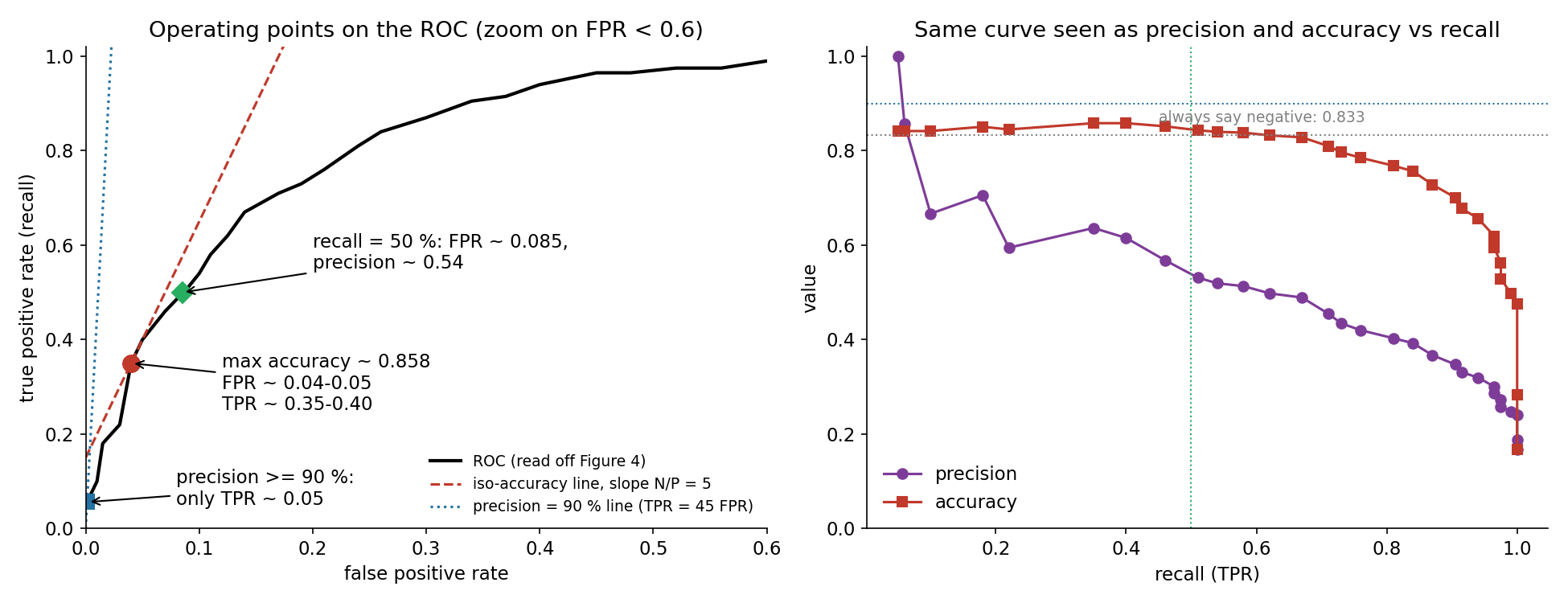
With $P = 200$ positives and $N = 1000$ negatives, every point $(\text{FPR}, \text{TPR})$ fixes the confusion matrix: $TP = 200\,\text{TPR}$, $FP = 1000\,\text{FPR}$.

(a) Maximum accuracy. $\text{acc} = (200\,\text{TPR} + 1000(1-\text{FPR}))/1200$, so we maximise $200\,\text{TPR} - 1000\,\text{FPR}$. Lines of equal accuracy have slope $N/P = 5$: the best point is where a line of slope 5 touches the curve. That happens at the end of the steep initial part, around FPR $\approx$ 0.04 to 0.05, TPR $\approx$ 0.35 to 0.40, threshold $\approx$ 0.75 (light green on the colour bar), for an accuracy of about $0.858$. Note how little this beats the trivial "always negative" classifier ($1000/1200 = 0.833$): with a 1:5 imbalance, accuracy prefers very cautious thresholds.

(b) Maximum recall with precision $\ge$ 90 %. $\text{prec} = \frac{200\,\text{TPR}}{200\,\text{TPR} + 1000\,\text{FPR}} \ge 0.9 \iff \text{TPR} \ge 45\,\text{FPR}$: the point must lie above a very steep line through the origin. The curve only satisfies this at its very start, where FPR is essentially 0: TPR $\approx$ 0.05 (about 10 of 200 positives), FPR $\approx$ 0, threshold $\approx$ 0.9 (the highest, yellow). Already at TPR 0.10 the curve has FPR $\approx$ 0.01, i.e. 10 false positives for 20 true ones (precision 0.67). This classifier simply cannot deliver 90 % precision at a useful recall.

(c) Maximum precision with recall $\ge$ 50 %. On a concave ROC curve precision decreases as we move right, so take the leftmost point with TPR $\ge 0.5$: TPR $\approx$ 0.50, FPR $\approx$ 0.085, threshold $\approx$ 0.65 to 0.7. Precision $= 100/(100+85) \approx 0.54$.

B3. Output activation and loss

1. (a) Binary classification: one output with sigmoid, binary cross-entropy (in PyTorch, raw logit + BCEWithLogitsLoss, which is numerically stabler). (b) 5-class single-label: 5 outputs with softmax, categorical cross-entropy (CrossEntropyLoss on raw logits, which applies log-softmax internally). (c) Unbounded regression: linear (identity) output, MSE (or MAE/Huber if outliers matter).
2. ReLU before binary cross-entropy is broken in three ways. Its output lies in $[0, \infty)$, not in $(0,1)$: it is not a probability, and $\log(1-\hat p)$ is undefined for $\hat p \ge 1$. An output of exactly 0 gives $\log 0 = -\infty$ when the label is 1. And for negative pre-activations the gradient is exactly 0, so a positive example predicted at 0 sends no learning signal back ("dead" output), so the network cannot fix its mistakes.

B4. Gradient descent variants and vanishing gradients

1. With $n = 60\,000$ images:

	batch GD	stochastic GD (1 sample)	mini-batch GD (e.g. 64)
(a) updates per epoch	1	60 000	about 940
(b) cost per update	whole dataset (high memory, slow)	one sample (cheap, but cannot use vectorised hardware)	one batch (fits GPU well)
(c) convergence	smooth, exact gradient, but very slow progress per unit of compute; can stall in sharp minima or saddle points	very noisy path, needs a decaying learning rate; noise can help escape poor regions	good compromise: reduced noise, many updates, standard in practice

2. (a) Vanishing gradients. (b) Backpropagation multiplies, layer after layer, the local derivatives of the activations and the weight matrices (chain rule). If those factors are smaller than 1 (saturating sigmoid/tanh have derivatives at most 0.25 and 1, small initial weights, ReLU units that are inactive so their derivative is 0), the product shrinks geometrically with depth, so early layers barely learn. (c) Mitigations: ReLU-family activations (Leaky ReLU, GELU) to avoid saturation and dead units; proper initialisation (He/Xavier); batch or layer normalisation; residual (skip) connections; for recurrent networks, LSTM/GRU; adaptive optimisers and a suitable learning rate help a little. (For the 3-layer network described, the usual culprit is dying ReLU units or a poor initialisation, so Leaky ReLU and He initialisation are the first fixes.)

B5. Self-attention and cross-attention calls

# (a) self-attention: queries, keys and values all come from the decoder input
attn_output1, _ = self.self_attn(decoder_input, decoder_input, decoder_input,
                                 attn_mask=decoder_mask)
# (b) cross-attention: queries from the decoder, keys and values from the retrieved documents
attn_output2, _ = self.cross_attn(attn_output1, doc_embeddings, doc_embeddings,
                                  key_padding_mask=doc_mask)

nn.MultiheadAttention(embed_dim, num_heads) is called as (query, key, value, ...) with tensors of shape (seq_len, batch, dim) by default (batch_first=False), which matches the docstring. attn_mask (a causal mask of shape (L, L)) stops a decoder position from looking at future tokens; for the documents the mask usually marks padded positions, which is key_padding_mask of shape (batch, doc_seq_len) (if doc_mask is an (L, S) mask, pass it as attn_mask instead). Two remarks a careful reader should make: the constructor's arguments are named d_model, nhead but the body uses hidden_dim, num_heads (should be nn.MultiheadAttention(d_model, nhead)), and a real decoder block would add residual connections and layer normalisation around each attention.

2. Why the query comes from the decoder. The query expresses "what this output position needs to know"; keys describe what each piece of retrieved text is about, and values carry the content to copy. Each decoder position therefore scores all document tokens against its own need and takes a weighted mix of their content. The output has one vector per decoder position, which is what the next layers and the token predictions need. Swapping the roles would produce one vector per document token, i.e. a re-encoding of the documents, not a decoder that reads them.

B6. Which LoRA configuration to deploy

Final validation losses (epoch 5, read off Figure 5): A $\approx 0.4215$, B $\approx 0.4087$, C $\approx 0.4003$. The 5 % tolerance around the best is $0.4003 \times 1.05 = 0.4203$.

• C is the best but has the most trainable parameters (8M) and adapts 4 matrices.
• B is 2.1 % worse than C, inside the tolerance, with half the parameters (4M).
• A is 5.3 % worse: just outside the tolerance, despite being the smallest.

Choose B: the smallest configuration that meets the quality requirement, which is what a memory-limited, low-latency deployment asks for. A nuance worth adding: LoRA adapters can be merged into the base weights ($W' = W + BA$) before deployment, after which every configuration has the same latency and memory as the base model. The size difference then matters only if adapters are kept separate (e.g. several adapters served on one base model), which is when B's smaller footprint pays off.

B7. Brain tumour segmentation

1. U-Net. The task is pixel-level segmentation, and U-Net outputs one label per pixel; its encoder-decoder with skip connections combines context with precise localisation, and it was designed for biomedical images with small datasets. YOLOv5 gives bounding boxes (detection), not masks; CLIP gives image-level embeddings aligned with text, with no dense output.
2. Two extra pooling layers enlarge the receptive field (more context, which can help with large tumours) but shrink the bottleneck from $32\times 32$ to $8\times 8$ for a 512 input. Fine detail (small lesions, boundaries) is lost in the deep features and must be recovered by the decoder from skip connections, so boundary accuracy and small-tumour recall typically drop; the model also gets more parameters and is easier to overfit on a small medical dataset. Net effect on segmentation quality: usually worse unless the images contain mostly large structures.
3. Each pooling halves each side: $512 / 2^4 = 32$, so the feature map is $32 \times 32$ (with the number of channels set by the last convolution).

B8. Text to sketch to photo

1. Yes, in principle, with a text-conditional GAN (StackGAN, AttnGAN, GigaGAN): the generator takes noise plus a text embedding, and the discriminator judges image-text pairs. An unconditional GAN cannot, since it has no way to receive the prompt. In practice large diffusion or autoregressive models such as DALL-E follow open-ended compositional prompts ("elderly woman", "watering", "garden") much better, because they are trained on huge image-text corpora and are more stable to train; GANs are prone to mode collapse and are usually trained on narrow domains.
2. Pix2Pix needs paired, pixel-aligned examples: (sketch, photo) pairs of the same scene. The usual trick is to create them synthetically, by running an edge or line-drawing extractor (Canny, HED, a sketch filter) on real photos of people and gardens, so that the input domain matches the style DALL-E will produce. Without paired data one would use an unpaired method such as CycleGAN.

Section C: ML Applications

C1. Spoiled produce detection

1. Extra data. More crate images with masks, covering many vegetable types, lighting, camera angles, crate types and stages of spoilage (early spoilage is the hard case); masks of fresh produce too (or at least instance boundaries) so the model learns to separate touching vegetables; time series of the same crate (spoilage evolves); hard negatives (dirt, natural blemishes, shadows). Synthetic: yes, by augmentation (colour, blur, rotation), copy-paste of segmented spoiled vegetables onto fresh crates, and generative models or rendering to create spoilage patterns; semi-supervised pseudo-labels on the unlabelled part of the dataset.
2. Approach (abstract components). Image capture and preprocessing (normalisation, colour correction) then instance segmentation of individual vegetables, then spoilage classification or segmentation per instance (or directly a two-class instance segmentation "spoiled / fresh"), then post-processing: convert masks to polygons (contour extraction and simplification), filter by confidence and minimum area, then display. Optionally temporal tracking across periodic images to confirm spoilage and avoid flicker.
3. Model choices. Instance segmentation: Mask R-CNN, YOLOv8-seg, or SAM prompted by a detector; semantic segmentation of spoiled areas: U-Net or DeepLabV3 with a pretrained backbone; per-instance classifier: a fine-tuned ResNet/EfficientNet/ViT on crops; polygons: OpenCV findContours + Douglas-Peucker simplification; semi-supervision: teacher-student pseudo-labelling.
4. Metrics. Mask IoU / Dice per spoiled item and mask mAP (at IoU 0.5 and 0.5:0.95) for localisation quality; at the item level recall of spoiled vegetables (missing one spoils neighbours) together with precision (staff time wasted on false alarms), possibly an $F_2$; an operational measure such as staff time saved or waste reduced.

C2. Prescription digitisation

1. Extra data. Word- or line-level transcriptions and bounding boxes of medicine lines (not just the final cart), a list of common abbreviations and generic-to-brand mappings, handwriting samples of many doctors, prescriptions mentioning medicines absent from the catalogue (needed to learn the "not found" case), and records of past human-expert corrections. Synthetic: yes, render printed and handwritten-style prescriptions from catalogue entries with handwriting fonts or a handwriting generator, with noise, stamps, skew and scanning artefacts; text-level augmentation with misspellings and abbreviations ("tab", "mg").
2. Approach. Image preprocessing (deskew, denoise) then layout analysis / text detection (find medicine lines) then handwriting and printed text recognition (OCR/HTR) then information extraction: tag brand name, dosage form, strength in each line (named-entity recognition) then catalogue matching / entity linking: fuzzy and semantic search of the extracted triple in the catalogue, with the strength and form as hard constraints, then confidence estimation and routing: if OCR confidence, match score or consistency checks are low, send to a human; if no catalogue match is close enough, output the extracted name with "no matching product".
3. Model choices. Text detection: CRAFT, DBNet, or a layout model (LayoutLMv3); recognition: TrOCR, PaddleOCR, Tesseract for printed text; or one end-to-end document model (Donut, or a vision-language model prompted to return JSON). Extraction: fine-tuned BERT/BioBERT token classifier or an LLM with constrained output. Matching: edit distance (Levenshtein) and phonetic matching on brand names plus embedding similarity (sentence embeddings + nearest-neighbour index); a learned re-ranker. Confidence: calibrated scores (temperature scaling) with a threshold tuned for the target error rate.
4. Metrics. Character/word error rate for OCR; precision, recall and F1 of extracted cart items (an item counts only if brand, form and strength are all correct: a wrong strength is a safety issue); accuracy on the "not in catalogue" cases; and for routing, the automation rate vs error rate among automated prescriptions (risk-coverage curve), since the business wants as few human reviews as possible at a very low error rate.

C3. Automated exam scoring

1. Extra data. The key missing piece is human scores with rubric-point explanations for a sample of responses, ideally from two graders to measure inter-rater agreement (the ceiling for any system). Also: examples of each score level per question, known edge cases (off-topic, copied model answer, very short answers), and demographic or school metadata to audit bias. Synthetic: yes, an LLM can generate responses of controlled quality (perturbing the model answer, injecting grammar errors, omitting rubric points) to create graded training and test data, but final evaluation must be on real human-graded responses.
2. Approach. Route by question type: (a) grammar correction: compare the student's correction with the reference using edit-level alignment (which errors were fixed, which new errors introduced); (b) factual / interpretive: check each rubric point for presence in the answer (entailment of the rubric points by the response); (c) essays: score each rubric dimension (content, organisation, language) separately. Then score aggregation following the rubric, and explanation generation that cites the rubric criteria and the evidence spans in the response. Add consistency and safety layers: calibration against human scores, uncertainty-based routing of borderline cases to a human, and bias audits.
3. Model choices. LLM-as-a-judge prompted with question, model answer, rubric and a few graded examples (structured JSON output, low temperature, several samples averaged for stability); fine-tuned cross-encoders (BERT/DeBERTa) for rubric-point entailment and for score regression once human scores exist; grammar: ERRANT-style edit extraction and a grammatical error correction model; similarity features: sentence embeddings between response and model answer; ordinal regression or gradient boosting to combine features into the final score.
4. Metrics. Agreement with human graders: quadratic weighted kappa (the standard for essay scoring, it penalises large disagreements more), Pearson/Spearman correlation and exact or adjacent agreement; compare with human-human agreement. Per-rubric-point precision and recall for the explanations; robustness tests (prompt injection in answers, length manipulation, paraphrases of the model answer); fairness: score gaps across student groups at equal human score.

What to remember

• Read code by tracking shapes and keys. Merges drop rows by key semantics (left keeps left keys, inner keeps matches), and tensor code is right when every intermediate shape is right; write them down.
• Accuracy is almost never the right metric under imbalance. Use recall, precision, PR-AUC; choose the operating point from the costs (iso-accuracy lines have slope $N/P$, precision constraints are lines $\text{TPR} = c\cdot\text{FPR}$ through the origin), and correct probabilities when the class priors change between training and deployment.
• Match the inductive bias to the data shape: interactions and blobs suit trees and k-means, rings suit RBF kernels and spectral clustering, and pure noise calls for a simple regularised model and cleaning, not a more flexible one.
• Derive the classic closed forms once and keep them: $\nabla(x^\top Bx) = (B+B^\top)x$, the softmax Jacobian $\mathrm{diag}(p) - pp^\top$, projection onto a hyperplane, and ridge-like minimisers $(mM+\lambda I)^{-1}M\sum u_i$; then check them numerically.
• System design answers follow one template: data you lack (and what can be synthesised), a pipeline of abstract components, concrete models per component, and metrics that match the real cost of errors, including when to hand over to a human.