Theory Problems

The problem in brief

The theory section of the 2025 Indian AI Olympiad (Stage 2) has three problems of 8 points each.

1. Exam scores as random variables. A student's score $X$ and an AI assistant's score $Y$ are correlated Gaussians, $U$ is a uniform adjustment and $V$ a discrete triangular bonus. You must reason about the distributions of their combinations.
2. Debt resolution on a graph. A person in debt $b$ receives $b$ from each of their $k$ friends, which leaves them with $b(k-1)$. Solve a chain example, prove that chains and trees can always be cleared when the total is non-negative, and find a counterexample on complete graphs.
3. Social-media response times. Model them with Gamma distributions: maximum-likelihood estimates, whether K-means suits the data, a Bayes classifier between two groups, and the meaning of the Gamma parameters.

How you are scored

Answers are typed into a form. Numeric answers must match the key (integers rounded down, decimals to two places), and justifications earn separate points; expressions are graded generously. No answer key is published, so all answers below are derived here and checked numerically in solution.py. Throughout we assume that $U$ and $V$ are independent of each other and of $(X, Y)$, and that $(X, Y)$ is jointly Gaussian; the statement only says "correlated".

The key idea

• Problem 1: variances add over independent terms, with a $2\rho\sigma_X\sigma_Y$ correction for correlated ones; adding a discrete variable to a Gaussian gives a finite Gaussian mixture.
• Problem 2: total wealth is preserved by every donation. On trees, a leaf can be merged into its neighbour: induction on the number of nodes. On complete graphs, pairwise differences modulo $n$ are invariant, which blocks some configurations forever.
• Problem 3: a Bayes decision boundary is where $\log p_G + \log f_G(x) = \log p_T + \log f_T(x)$. For Gamma densities this is linear in $x$ and in $\log x$, so it is a straight line exactly when the shapes are equal.

The full solution

Problem 1: score distributions

Q1(a). The ideal family. With $N$ problems scoring $+1$ (correct), $0$ (skipped) or $-0.5$ (wrong), $X = C - 0.5\,W$, where $C$ and $W$ count correct and wrong answers. If the problems are i.i.d. with probabilities $(p_c, p_s, p_w)$, then $(C, S, W) \sim \mathrm{Multinomial}(N; p_c, p_s, p_w)$, so $X$ is an affine function of a multinomial vector. It is discrete, bounded in $[-N/2, N]$, with mean $N(p_c - 0.5 p_w)$ and variance $N\big(p_c + 0.25 p_w - (p_c - 0.5 p_w)^2\big)$. With problems of unequal difficulty it becomes a sum of independent non-identical categorical variables (Poisson-multinomial type).

Q1(b). Is the Gaussian appropriate? As an approximation, yes, when $N$ is large and the probabilities are not extreme: $X$ is a sum of $N$ independent bounded terms, so the central limit theorem applies. But it is only an approximation: the true score is discrete and bounded, and it is skewed for very strong or very weak students (near the ceiling or the floor), where a Gaussian puts mass on impossible scores.

Q2(a). For jointly Gaussian $(X, Y)$, any linear combination is Gaussian:

$$Z = X - Y \sim \mathcal N\big(\mu_X - \mu_Y,\ \sigma_X^2 + \sigma_Y^2 - 2\rho\,\sigma_X\sigma_Y\big).$$

Q2(b). Replace $\sigma_X^2$ by $\sigma_X^2/\alpha$ and $\sigma_Y^2$ by $\alpha\sigma_Y^2$, with $\rho$ unchanged. The standard deviations become $\sigma_X/\sqrt\alpha$ and $\sqrt\alpha\,\sigma_Y$, so their product, and hence the covariance term, does not change. The variance of $Z$ is unchanged if and only if

$$\frac{\sigma_X^2}{\alpha} + \alpha\sigma_Y^2 = \sigma_X^2 + \sigma_Y^2 \iff (1 - \alpha)\left(\frac{\sigma_X^2}{\alpha} - \sigma_Y^2\right) = 0,$$

that is $\alpha = 1$ (no change) or $\alpha = \sigma_X^2/\sigma_Y^2$ (the two variances swap). It does not depend on $\rho$, because the term $-2\rho\sigma_X\sigma_Y$ is the same before and after.

Q2(c).

$$\operatorname{Var}(3X - 2Y) = 9\sigma_X^2 + 4\sigma_Y^2 - 12\rho\sigma_X\sigma_Y = 36 + 64 - 76.8 = \mathbf{23.2}$$

(23 in the integer format). The means play no role; a simulation of $10^6$ draws gives 23.23.

Q3(a). $X + U$. The convolution of the Gaussian density with the uniform density on $[a - T, a + T]$ gives

$$f_{X+U}(s) = \frac{1}{2T}\left[\Phi\!\left(\frac{s - \mu_X - a + T}{\sigma_X}\right) - \Phi\!\left(\frac{s - \mu_X - a - T}{\sigma_X}\right)\right],$$

a "smoothed box", with mean $\mu_X + a$ and variance $\sigma_X^2 + T^2/3$ (the uniform on an interval of length $2T$ has variance $(2T)^2/12$).

Q3(b). Increasing $T$ leaves the mean $\mu_X + a$ unchanged and increases the variance quadratically, by $T^2/3$; the density becomes flatter and wider.

Q3(c). $X + V$. Write $V = b + j$. The probabilities are $w_j = (D - |j|)/D^2$ for $|j| \le D$; the two end points have weight 0, and the weights sum to 1. Conditioning on $V$:

$$f_{X+V}(s) = \sum_{j=-(D-1)}^{D-1} \frac{D - |j|}{D^2}\cdot\frac{1}{\sigma_X}\,\varphi\!\left(\frac{s - \mu_X - b - j}{\sigma_X}\right),$$

with mean $\mu_X + b$ and variance $\sigma_X^2 + \frac{D^2 - 1}{6}$, because

$$\operatorname{Var}(V) = \frac{2}{D^2}\sum_{j=1}^{D-1} j^2 (D - j) = \frac{D^2 - 1}{6}.$$

Q3(d). It is a finite mixture of Gaussians: $2D - 1$ components with the same variance $\sigma_X^2$, means $\mu_X + b + j$ and triangular weights. It is a single Gaussian only in the degenerate case $D = 1$, where $V = b$ is constant.

Q3(e). By independence, $\operatorname{Var}(U + V) = \dfrac{T^2}{3} + \dfrac{D^2 - 1}{6}$ (simulated: 4.326 against 4.333 for $T = 3$, $D = 3$).

Q4. Final score with $a = b = 0$. Let $m = \mu_X - \mu_Y$ and $\sigma_Z^2 = \sigma_X^2 + \sigma_Y^2 - 2\rho\sigma_X\sigma_Y$. Combining the two previous results, $S = X - Y + U + V$ is a triangular mixture of "smoothed boxes":

$$f_S(s) = \sum_{|j| < D} \frac{D - |j|}{2T D^2}\left[\Phi\!\left(\frac{s - m - j + T}{\sigma_Z}\right) - \Phi\!\left(\frac{s - m - j - T}{\sigma_Z}\right)\right],$$

with mean $m$ and variance $\sigma_Z^2 + T^2/3 + (D^2 - 1)/6$.

Problem 2: debt resolution

A donation at $X$ (debt $b$, $k$ friends) adds $kb$ to $X$ and removes $b$ from each friend, so the total is invariant. A configuration with negative total can therefore never be cleared, which is why the statement requires total $\ge 0$.

Q1. The chain $(+3, -4, -2, +5, -1)$ (Anu, Ben, Cam, Dan, Eva), total $+1$. A breadth-first search over all legal sequences gives a shortest solution of 8 donations:

donation at	Anu	Ben	Cam	Dan	Eva
start	3	-4	-2	5	-1
Ben	-1	4	-6	5	-1
Anu	0	3	-6	5	-1
Cam	0	-3	6	-1	-1
Ben	-3	3	3	-1	-1
Anu	0	0	3	-1	-1
Eva	0	0	3	-2	0
Dan	0	0	1	2	-2
Eva	0	0	1	0	0

Q2 and Q3. Chains and trees. A chain is a tree, so we prove the tree statement; for a chain, "leaf" simply means "end node". The proof is by induction on $n$, for any configuration with total $s \ge 0$.

Base case. For $n = 1$, the single value equals $s \ge 0$: nothing to do.

Inductive step. Take a leaf $L$ (it exists for $n \ge 2$) with its unique neighbour $P$, and let $T' = T \setminus \{L\}$, again a tree, with $n - 1$ nodes. In $T'$, give $P$ the merged value $P' = P + L$; the total of $T'$ is still $s$.

Case A: $L \le 0$. If $L < 0$, donate at $L$: $L$ becomes $0$ and $P$ loses $|L|$, so now $L = 0$ and $P = P'$. By induction there is a finite sequence clearing $T'$. Replay it in $T$:

• a donation at a node other than $P$ is identical in $T$ and $T'$ (the leaf is not its friend);
• a donation at $P'$ (debt $b'$, $k'$ friends in $T'$) becomes two moves in $T$. First donate at $P$, whose debt is also $b'$: $P$ gets $k'b'$, its $T'$-friends lose $b'$ each, and $L$ goes to $-b'$. Then donate at $L$: $L$ returns to $0$ and $P$ loses $b'$. The result is $P = (k' - 1)b'$, exactly as in $T'$, with $L = 0$.

So the replay keeps $L = 0$ and $P = P'$; when $T'$ is cleared, all of $T$ is.

Case B: $L = c > 0$. Replay the sequence of $T'$ as before; while $P$ never donates, $L$ stays equal to $c$ and $P = P' - c$. Two events can interrupt the replay.

• $T'$ asks $P'$ to donate. Do the same two moves as in case A ($P$'s debt is now $b' + c$). Afterwards $L = 0$: the new configuration of $T'$ is not the planned one, but it still has total $s \ge 0$. We restart in case A, which terminates.
• The sequence of $T'$ ends with $P' \ge 0$ but $P = P' - c < 0$. Then donate at $P$: its debt $b = c - P'$ satisfies $0 < b \le c$, so $L$ becomes $c - b = P' \ge 0$, which is strictly smaller than $c$. We restart case B with this smaller reserve.

The reserve $c$ is a non-negative integer that strictly decreases at each restart of the second kind, and a restart of the first kind leads to case A. So after finitely many rounds everything is debt-free. $\blacksquare$

solution.py implements exactly this recursive procedure and clears all debts on 3,000 random trees (up to 9 nodes, values in $[-7, 7]$, total $\ge 0$).

Q4. A counterexample on $K_n$. In the complete graph, every node is everyone's friend. A donation at $X$ with debt $b$ subtracts $b$ from every node and adds $nb$ to $X$. Hence every pairwise difference $v_i - v_j$ is invariant modulo $n$. Take

$$v = (-1,\ 0,\ 1,\ 2,\ \dots,\ n - 2), \qquad s = \frac{(n-1)(n-2)}{2} - 1 \ge 0 \quad (n \ge 3).$$

The $n$ values are pairwise distinct modulo $n$, and they stay so forever. A debt-free configuration with $n$ distinct residues has total at least $0 + 1 + \dots + (n - 1) = \frac{n(n-1)}{2}$, which is larger than $s$. Since the total is preserved, the debts can never all be cleared, whatever the order of donations. An exhaustive search confirms that no sequence clears $(-1, 0, 1)$ on $K_3$, $(-1, 0, 1, 2)$ on $K_4$, or $(-1, 0, \dots, 3)$ on $K_5$. The idea is the same as the "genus" of the graph in chip-firing: trees have none, complete graphs have cycles that create obstructions.

Problem 3: response times

Q1(a). Exponential case ($k = 1$).

$$\ell(\theta) = -n\log\theta - \frac{1}{\theta}\sum_i x_i, \qquad \ell'(\theta) = -\frac{n}{\theta} + \frac{\sum x_i}{\theta^2} = 0 \Rightarrow \hat\theta = \bar x,$$

the sample mean of the response times. It is a maximum, since $\ell''(\hat\theta) = -n/\bar x^2 < 0$.

Q1(b). Both parameters free. The log-likelihood is

$$\ell(k, \theta) = (k - 1)\sum_i \log x_i - \frac{1}{\theta}\sum_i x_i - nk\log\theta - n\log\Gamma(k).$$

Setting $\partial\ell/\partial\theta = 0$ gives $\hat\theta = \bar x / k$. Substituting into $\partial\ell/\partial k = 0$, i.e. $\sum\log x_i - n\log\theta - n\psi(k) = 0$, gives

$$\log\hat k - \psi(\hat k) = \log\bar x - \overline{\log x},$$

where $\psi$ is the digamma function and $\overline{\log x}$ the mean of $\log x_i$. There is no closed form, but the left side decreases strictly from $+\infty$ to $0$, so there is a unique root (Newton's method; a good start is $k_0 \approx \frac{3 - s + \sqrt{(s-3)^2 + 24 s}}{12 s}$, with $s$ the right side). The right side is $\ge 0$ by Jensen's inequality. Then $\hat\theta = \bar x/\hat k$. On a simulated Gamma(2.5, 3) sample this recovers $\hat k = 2.497$, $\hat\theta = 3.005$.

Q2(a). Does vanilla K-means converge? Yes, to a local minimum (a fixed point) in a finite number of steps. Neither the assignment step nor the update step increases $J$, and there are finitely many partitions, so with a fixed tie-breaking rule no partition repeats. The local minimum need not be global and depends on the initialisation (an empty cluster must be handled, for example by re-seeding it).

Q2(b). Should it be modified? Yes. Response times are positive and right-skewed, and the groups differ mainly in scale: GenX times are larger and more spread, since the variance $k\theta^2$ grows with $\theta$. Squared Euclidean distance assumes round clusters of similar spread, so the slow, dispersed group gets split while the fast groups merge. Reasonable fixes:

• log-transform the times (a scale change becomes a shift, and skewness drops), and standardise the two apps;
• use a Bregman divergence matched to the Gamma family. For a fixed shape this is the Itakura-Saito divergence $d(x, c) = \frac{x}{c} - \log\frac{x}{c} - 1$, and the centroid is still the mean (Banerjee et al., 2005);
• or, best, fit a mixture of Gamma distributions with EM (soft assignments, a $(k, \theta)$ pair and a prior per group), which is exactly the model used in Q3.

Q3(a). Teen or GenX? Use the Bayes rule. Treat the two apps as independent given the group (the product form of the multivariate Gamma above), with log-density

$$\log f_g(x) = \sum_{a \in \{W, I\}} \Big[(k_{a,g} - 1)\log x_a - \frac{x_a}{\theta_{a,g}} - k_{a,g}\log\theta_{a,g} - \log\Gamma(k_{a,g})\Big].$$

Predict GenX when $\log p_G + \log f_G(x) > \log p_T + \log f_T(x)$. The boundary is

$$\sum_{a} \Big[(k_{a,G} - k_{a,T})\log x_a - \Big(\tfrac{1}{\theta_{a,G}} - \tfrac{1}{\theta_{a,T}}\Big)x_a\Big] + C = 0,$$

where $C = \log\frac{p_G}{p_T} + \sum_a\big[k_{a,T}\log\theta_{a,T} + \log\Gamma(k_{a,T}) - k_{a,G}\log\theta_{a,G} - \log\Gamma(k_{a,G})\big]$.

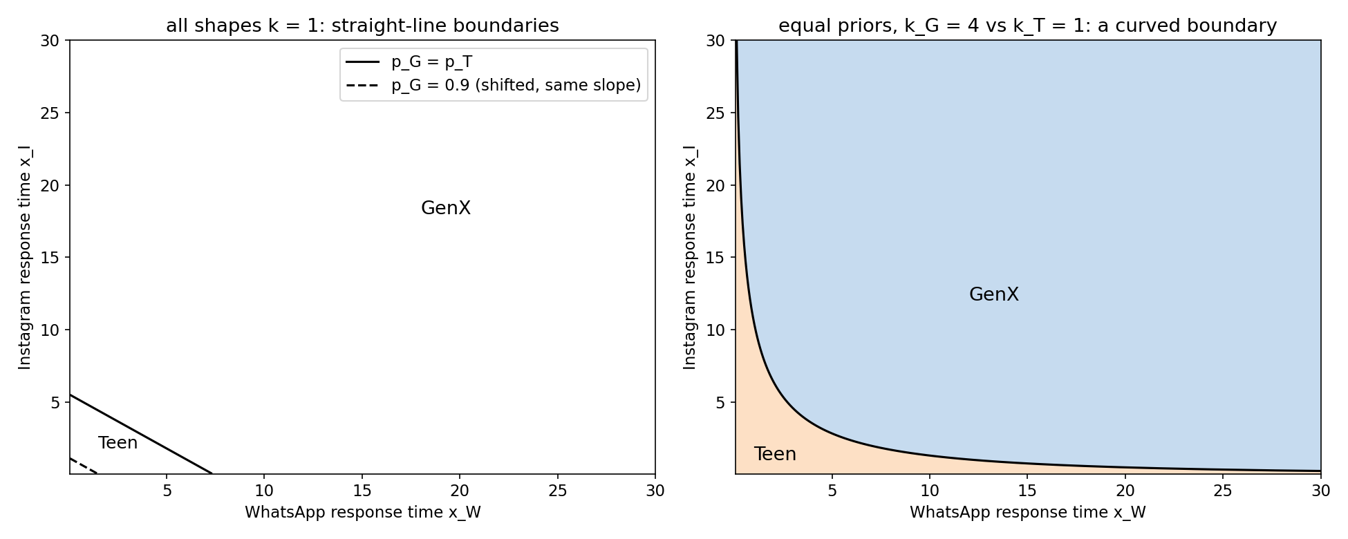
Q3(b). All shapes equal to 1. The $\log x$ terms vanish and the boundary $\sum_a (1/\theta_{a,T} - 1/\theta_{a,G})\,x_a = \text{const}$ is a straight line. Equal priors give one particular line; unequal priors only change the constant by $\log(p_G/p_T)$, which yields a parallel line shifted towards the less likely group.

Q3(c). Equal priors, different shapes. The $\log x_a$ terms remain, so the boundary is curved (a level set of a sum of terms $\alpha\log x - \beta x$). When the GenX group has both the larger shape and the larger rate ($\alpha, \beta > 0$), each term is concave with a maximum at $x = \alpha/\beta$, and the GenX region becomes a bounded convex set enclosed by a closed curve.

Q4(a). Since the mean is $k\theta$ and the variance $k\theta^2$, "much longer" WhatsApp replies for GenX mean $k_{W,G}\theta_{W,G} \gg k_{W,T}\theta_{W,T}$. The natural reading is a larger scale $\theta_{W,G} > \theta_{W,T}$ (slower and more spread out), with comparable shapes; a larger $k_{W,G}$ would also raise the mean, but it would make the GenX times relatively more regular.

Q4(b). On Instagram, Teens are faster (smaller mean $k\theta$) and more consistent. The coefficient of variation of a Gamma is $1/\sqrt k$, so more consistency means a larger shape $k_{I,T} > k_{W,T}$, and a much smaller scale $\theta_{I,T} \ll \theta_{W,T}$ to bring the mean down to seconds or minutes. On WhatsApp the Teen distribution is closer to exponential ($k \approx 1$, coefficient of variation near 1, heavy right tail) with a large $\theta$.

Results

question	answer
P1 Q1	multinomial (affine), Gaussian only as a large-$N$ approximation
P1 Q2	$Z \sim \mathcal N(\mu_X - \mu_Y, \sigma_X^2 + \sigma_Y^2 - 2\rho\sigma_X\sigma_Y)$; unchanged iff $\alpha \in \{1, \sigma_X^2/\sigma_Y^2\}$, independent of $\rho$; $\operatorname{Var} W = 23.2$
P1 Q3	$X + U$: Gaussian convolved with a uniform, variance $+T^2/3$; $X + V$: mixture of $2D - 1$ Gaussians, variance $+(D^2 - 1)/6$; $\operatorname{Var}(U + V) = T^2/3 + (D^2 - 1)/6$
P1 Q4	triangular mixture of smoothed boxes, mean $\mu_X - \mu_Y$, variance $\sigma_Z^2 + T^2/3 + (D^2 - 1)/6$
P2 Q1	Ben, Anu, Cam, Ben, Anu, Eva, Dan, Eva (8 donations, final $(0, 0, 1, 0, 0)$)
P2 Q2-Q3	induction by merging a leaf into its neighbour (verified on 3,000 random trees)
P2 Q4	$(-1, 0, 1, \dots, n - 2)$: residues mod $n$ are invariant
P3 Q1	$\hat\theta = \bar x$; $\log\hat k - \psi(\hat k) = \log\bar x - \overline{\log x}$, $\hat\theta = \bar x/\hat k$
P3 Q2	converges to a local minimum; modify (log scale, Itakura-Saito, or Gamma-mixture EM)
P3 Q3	Bayes log-ratio boundary; linear when $k = 1$ (priors shift it), curved otherwise
P3 Q4	GenX on WhatsApp: larger $\theta$; Teens on Instagram: larger $k$, much smaller $\theta$

What to remember

• Look for invariants first. Total wealth (always) and differences modulo $n$ (on $K_n$) instantly tell you what is impossible.
• Induction on trees: remove a leaf. Merging a leaf into its neighbour, and simulating each of the neighbour's moves with one extra move at the leaf, is a reusable proof template.
• Correlated sums need the covariance term, and rescaling two variances by $\alpha$ and $1/\alpha$ leaves their covariance unchanged.
• Discrete plus Gaussian gives a Gaussian mixture; uniform plus Gaussian gives a smoothed box. Means and variances simply add for independent terms.
• Match the algorithm to the data's geometry. Skewed, scale-driven data calls for log transforms, the right divergence or a generative mixture, rather than plain Euclidean K-means; the Bayes boundary between exponential families is linear in their sufficient statistics ($x$ and $\log x$ for the Gamma).