SmogCast: Forecasting Air Pollution in Bangalore & Delhi

The problem in brief

You receive a weekly table for two Indian cities: PM2.5 pollution, average temperature and number of vehicles for Bangalore and for Delhi, plus a petrol price common to both. The training file covers 200 weeks. First you explore the data and answer three questions: are the two cities' pollution levels correlated, how does pollution relate to temperature and traffic, and does petrol price matter? Then you write two functions in the organisers' notebook: one that learns a forecasting model from the training file, and one that, given the history up to some week and the petrol prices of the coming weeks, predicts PM2.5 in both cities a few weeks ahead. Temperature and traffic for the future weeks are not given: only the week index and the petrol price are.

How you are scored

The notebook has a fixed evaluation cell. It takes a file, hides its last 12 weeks, gives your function everything before them, and asks for forecasts of the first lead_time = 6 hidden weeks. For each city it reports

$$\text{MAPE} = \frac{100}{n}\sum_{t=1}^{n}\left|\frac{y_t-\hat y_t}{y_t}\right| ,\qquad \text{MSE} = \frac{1}{n}\sum_{t=1}^{n}\left(y_t-\hat y_t\right)^2 ,\qquad n = 6 .$$

The cell is run on the training file and on a public test file; a private file is scored by the organisers. Points depend on "performance ranges" that were never published, so there is no official target number. The rest of the 14 points reward the exploration answers and a well-argued method.

Two details of the evaluation cell are worth noticing before writing any code:

• The public test file is the training file plus 100 new weeks (its first 200 rows are identical to the training file). The scored weeks are 289 to 294, forecast from history up to week 288. So "forecasting" here means 1 to 6 steps ahead.
• The model is trained with lead_time=3 but evaluated with lead_time=6. A model that only knows how to predict exactly 3 weeks ahead breaks. Our model must handle any horizon.
• Six weeks per city is a tiny sample: one unlucky week can double the MSE. To compare ideas fairly we also run a rolling backtest: we repeat the official procedure from each of the 95 origins between weeks 200 and 294 (all in the period never used for fitting) and average.

First look at the data

Plot everything against time first. Three structures appear immediately.

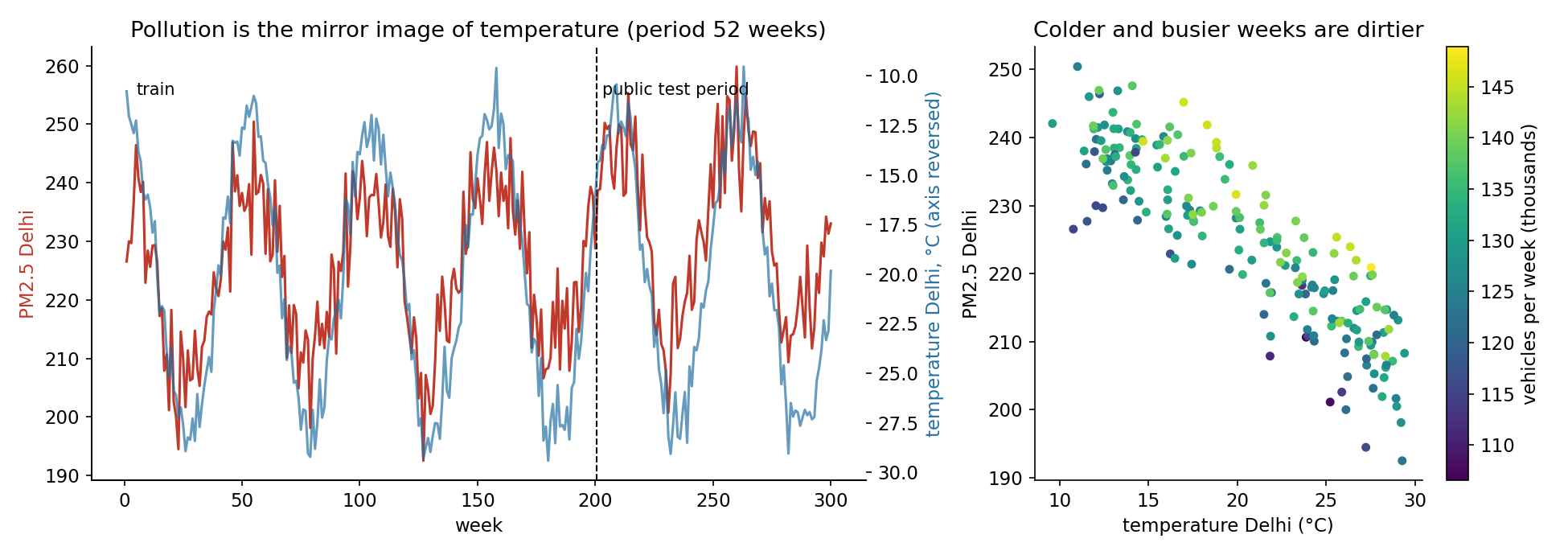
• Temperature is a clean yearly wave (period 52 weeks) plus small weekly noise of about 1 °C. Delhi swings between 10 °C and 29 °C, Bangalore between 21 °C and 29 °C.
• Traffic grows slowly (about 100 extra vehicles per week, every week), with noise that persists for a few weeks (lag-1 autocorrelation of the detrended series about 0.45).
• PM2.5 looks like the mirror image of temperature, plus noise. In Delhi, where the temperature swing is large, the seasonal wave dominates; in Bangalore it is weaker and the series looks noisier.

A linear regression of PM2.5 on the same week's temperature and traffic confirms this, and its residuals are pure white noise (lag-1 autocorrelation 0.01):

city	intercept	per °C	per 1000 vehicles	per INR of petrol	$R^2$
Bangalore	201.1	$-2.09$	$+0.39$	$+0.15$ (p = 0.41)	0.55
Delhi	204.5	$-1.96$	$+0.48$	$-0.04$ (p = 0.83)	0.87

Q1 (a): are the two cities correlated?

The honest answer is "yes, but not causally". The levels have a correlation of $r = 0.55$, which looks substantial. But both cities share the same calendar (winter is cold in both, $r = 0.88$ between their temperatures) and both see traffic grow over the years. Remove these common slow movements by looking at week-to-week changes, and the correlation vanishes:

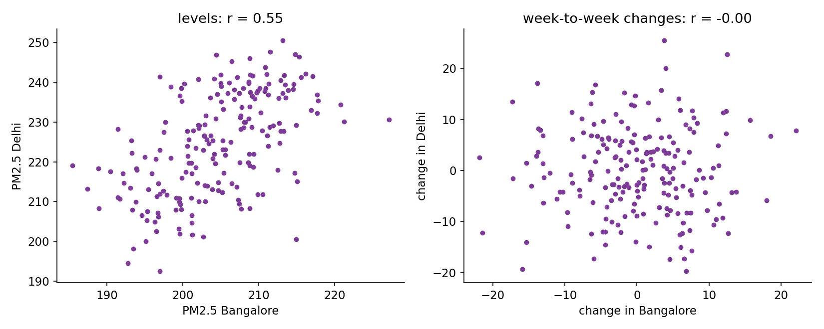
So knowing that Bangalore's pollution jumped this week tells you nothing about Delhi. The correlation of levels is a common-cause correlation (season and trend), exactly the trap that makes two trending time series look related. Practical consequence: there is no point feeding one city's PM2.5 into the other city's model.

Q1 (b): pollution, temperature and traffic

• PM2.5 decreases with temperature: about $-2$ units per °C in both cities (winter inversions trap particles near the ground; in this data the effect is very clean).
• PM2.5 increases with traffic: about $+0.4$ to $+0.5$ units per 1000 extra vehicles per week.
• Temperature and traffic are essentially uncorrelated with each other ($r \approx 0.05$): traffic follows the long-term trend, temperature the seasons. That is good news: the two effects can be estimated separately without confusion.

Q1 (c): petrol price

The raw correlation between petrol price and PM2.5 is tiny ($0.09$ and $-0.05$), and once temperature and traffic are in the regression its coefficient is indistinguishable from zero (p-values 0.41 and 0.83). So petrol has no direct effect. But it does act indirectly, through traffic: holding the trend and the season fixed, one extra rupee per litre removes about 1450 vehicles per week in Bangalore and 1690 in Delhi. Multiplied by the traffic effect, a 1 INR rise lowers PM2.5 by roughly $0.6$ in Bangalore and $0.8$ in Delhi. A careless reading of the raw correlation ("petrol rises over time and so does pollution, $r=0.18$ in the full file") would get this backwards: price and pollution both trend upward, while the causal path goes the other way.

A first baseline

The simplest forecasts need no model at all:

• last value: predict that every future week equals the last observed one;
• mean of the last 4 weeks: the same idea with less noise;
• same week last year: copy the value from 52 weeks earlier, to capture the season.

On the official public test window they give MAPE around 2.4 to 3.2 % and MSE 39 to 66, and on the rolling backtest MSE 46 to 107. They fail for clear reasons: the last value carries this week's random noise into the future, and last year's value carries last year's noise (and misses one year of traffic growth).

The notebook's helper code suggests XGBoost on lagged PM2.5 values, forecasting recursively. On the training file it looks brilliant (MSE 10.6 and 21.5), because the trees have memorised those very weeks. On the unseen weeks it is the worst model of all for Delhi (backtest MSE 122). Lags of PM2.5 carry little information here: the residual noise is white, so yesterday's value is mostly yesterday's noise, and recursive forecasting feeds predictions back in, compounding errors. This is the most useful failed attempt of the problem: always evaluate on weeks the model has not seen.

The key idea

Do not forecast pollution directly. Forecast its drivers, then use the physical relation.

The exploration shows that, week by week,

$$\text{PM}_t = a + b\,T_t + g\,V_t + \varepsilon_t ,\qquad \varepsilon_t \text{ white noise, sd } \approx 4.7 ,$$

with $T$ the temperature and $V$ the vehicle volume. The relation itself needs no forecasting; what is unknown at forecast time is $T_{t+h}$ and $V_{t+h}$. But these two are far easier to predict than PM2.5:

• Temperature is a seasonal curve. Fit it with yearly harmonics: $T_t \approx c_0 + c_1 \sin\frac{2\pi t}{52} + c_2 \cos\frac{2\pi t}{52} + c_3 \sin\frac{4\pi t}{52} + c_4 \cos\frac{4\pi t}{52}$ . The leftover noise is about 1 °C and does not persist, so this curve is the best possible forecast of $T_{t+h}$ for any horizon.
• Traffic is trend + season + petrol effect + a persistent shock. Fit $V_t = \text{(linear in } t\text{, harmonics, petrol}_t) + r_t$, where the residual follows $r_{t+1} \approx \varphi\, r_t + \text{noise}$ with $\varphi \approx 0.4$. The best forecast of a future shock is then $\varphi^h r_{\text{last}}$: if this week has unusually heavy traffic, the next week probably does too, and the effect fades geometrically.

The petrol price of the future weeks is given, so it enters exactly where it acts: in the traffic equation.

Why is this better than regressing PM2.5 on lags or on the calendar alone? Because it puts each piece of information in the right place. The calendar regression (PM2.5 directly on harmonics, trend and petrol) is already good, since it is almost the same model with the drivers substituted in. The structural version adds the persistence of traffic shocks, which the calendar cannot see, and it reads off interpretable coefficients that also answer Q1.

How good can anyone be? If we cheat and give the model the true future temperature and traffic, it still makes errors, because of $\varepsilon_t$: backtest MSE 23.6 (Bangalore) and 26.4 (Delhi). That is the noise floor of this data. Every forecast also pays for the unpredictable part of the drivers. Temperature noise (sd about 1 °C) adds about $b^2 \cdot 1^2 \approx 4$. A traffic shock $h$ weeks ahead is unpredictable up to a variance $\sigma_r^2(1-\varphi^{2h})$, which is almost $\sigma_r^2$ after two weeks; with $\sigma_r \approx 6000$ vehicles in Delhi this adds $(0.00048 \times 6000)^2 \approx 8$, and about $(0.00039 \times 4800)^2 \approx 3.5$ in Bangalore. Floor plus these terms gives roughly 31 (Bangalore) and 38 (Delhi); our model sits at 32.7 and 40.0: there is very little left to gain.

The full solution

1. Fit, on the 200 training weeks only, for each city:
   • the PM equation, linear regression of PM2.5 on $(T_t, V_t)$;
   • the temperature curve, linear regression of $T_t$ on $(t, \text{harmonics}, \text{petrol}_t)$;
   • the traffic curve, the same regression for $V_t$, and $\varphi$ = lag-1 autocorrelation of its residuals.
2. To forecast weeks $t+1, \dots, t+h$ from a history ending at week $t$:
   • compute the last traffic residual $r_t = V_t - \hat V_t$ from the history;
   • $\hat T_{t+k}$ = temperature curve at week $t+k$; $\hat V_{t+k}$ = traffic curve at week $t+k$ (with its known petrol price) $+\ \varphi^k r_t$;
   • plug into the PM equation.
3. Return a DataFrame with Week and Predicted_Particulate_Level_<city> columns, the names the evaluation cell merges on.

The heart of the forecasting function:

h = fut["Week"].to_numpy() - past_df["Week"].iloc[-1]            # 1..lead_time steps ahead
last_resid = (past_df[V] - veh_m.predict(calendar_features(past_df))).iloc[-1]
temp_f = temp_m.predict(X_fut)                                    # seasonal temperature
veh_f  = veh_m.predict(X_fut) + last_resid * phi ** h             # traffic, shock decays
pm_f   = pm_eq.predict(pd.DataFrame({T: temp_f, V: veh_f}))       # physical relation

Nothing is fitted on the test file: the history passed to the forecasting function is only used to read the last traffic shock, which any forecaster needs. (Refitting all equations on the longer history at forecast time, as the notebook's SARIMA helper does, changes the scores by less than 1 MSE unit: the 200 training weeks already pin the coefficients down.) Because the model forecasts any horizon, the mismatch between training (lead_time=3) and evaluation (lead_time=6) is harmless.

Results

Official evaluation cell on the public test file (weeks 289 to 294, 6 weeks), and rolling backtest over the 95 origins of the unseen period (weeks 200 to 294, horizons 1 to 6):

approach	official MAPE BLR	official MSE BLR	official MAPE DEL	official MSE DEL	backtest MSE BLR	backtest MSE DEL
last value	3.23 %	53.2	2.42 %	38.7	69.7	103.9
mean of last 4 weeks	2.92 %	45.4	2.49 %	38.8	45.8	107.4
same week last year	2.40 %	48.5	2.99 %	65.6	68.5	72.7
XGBoost on 4 lags + petrol (helper code)	1.78 %	18.2	2.34 %	50.6	51.4	122.3
calendar regression (harmonics + trend + petrol)	2.57 %	36.3	2.08 %	38.0	35.3	41.8
structural, no traffic persistence	1.97 %	21.1	2.13 %	36.8	32.8	40.6
structural (final)	1.97 %	21.1	2.18 %	36.9	32.7	40.0
noise floor: true future drivers given	1.27 %	10.1	2.27 %	31.9	23.6	26.4

On the official cell run on the training file (weeks 189 to 194, which the model has seen), the final model scores MAPE 1.96 % and 3.09 %, MSE 30.9 and 61.7.

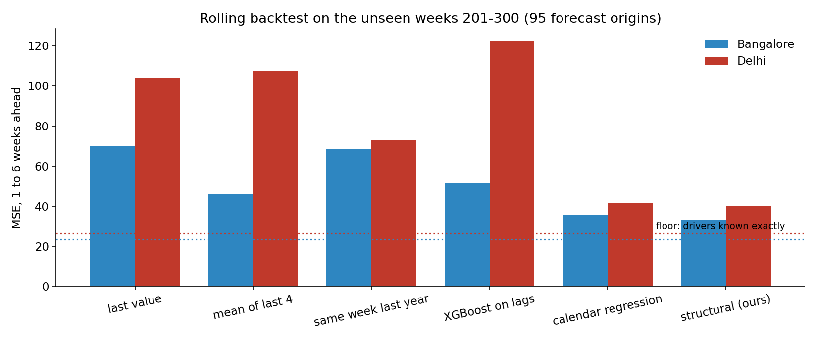
Look at the official columns with care: on Delhi the naive "last value" scores 38.7, almost the same as our 36.9, and even the oracle that knows the true future drivers has a worse Delhi MAPE (2.27 %) than our model. Six weeks are too few to rank models. The backtest, with 570 forecasts per city, separates them clearly: the structural model is the best of all honest forecasters and is within about 10 MSE units of the noise floor in both cities.

What to remember

• Forecast the drivers, not the target, when the target is a stable function of drivers that are themselves predictable (seasonal temperature, trending traffic). Put each known future input (here petrol price) in the equation where it really acts.
• Correlation between two trending or seasonal series is usually a common cause. Check by correlating week-to-week changes, or by controlling for the calendar, before concluding anything (Q1 a and c).
• Lags only help if the noise persists. Look at the autocorrelation of the residuals: white residuals mean past values of the target are mostly noise, and lag-based models (XGBoost, AR) will chase it.
• A 6-point test set is a lottery. Rebuild the official procedure as a rolling backtest over many origins, on data the model never saw, and compare models there.
• Estimate the noise floor (here: give the model the true future drivers). It tells you when to stop tuning.