IOAI Training: Learn AI by solving problems

The problem in brief

You receive 700 specimens of a fictional creature, each described by a capture location $(X, Y)$ , a body size and a diet (carnivore or herbivore). Only 50 of them carry their genetic strain (A, B, C or D); the other 650 are unlabelled. The notebook asks you to (1) explore whether location predicts the strain and whether k-means is a sensible way to find the strains, (2) write a location clustering function and measure how well its clusters match the known strains, (3) train a classifier on location and the other features, and (4) evaluate it on a fully labelled public test set of 50 specimens. A private test set was used by the organisers for a last point.

How you are scored

The rubric mixes written justifications and performance "ranges" that were not published. The two measured quantities are:

for the clustering, the normalised mutual information between clusters $C$ and known strains $S$ (computed on the 50 labelled specimens only), together with homogeneity and completeness:

\mathrm{NMI}(S, C) = \frac{2\, I(S; C)}{H(S) + H(C)}

where $I$ is the mutual information and $H$ the entropy. NMI is 1 when clusters and strains are in perfect one-to-one correspondence, and does not care about cluster names.

for the classifier, plain accuracy on the 50 public test specimens (and on the private set).

No threshold or reference score was published, so there is no target to compare with.

First look at the data

Plot the map before anything else. The left panel shows the 50 labelled specimens in colour over the 650 unlabelled ones in grey.

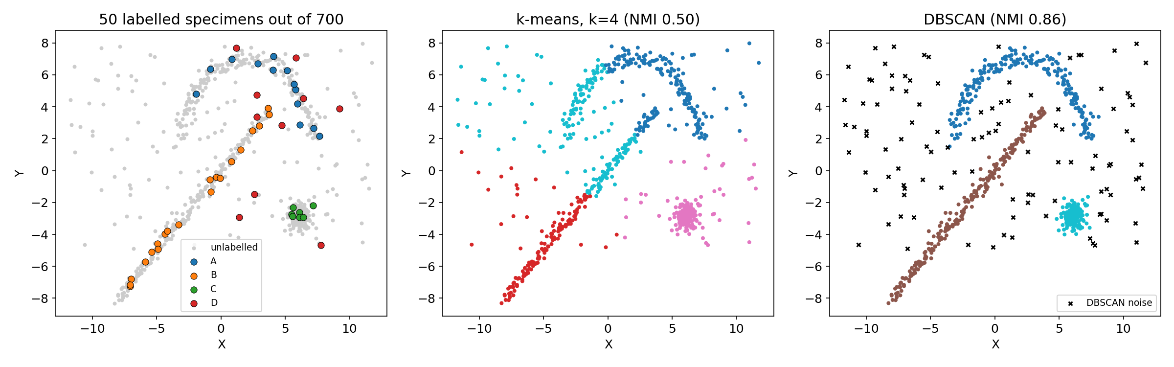
Left: labelled specimens on the map. Middle: k-means with k = 4. Right: DBSCAN, with its noise points as black crosses.

The terrain has a very clear shape: an arc at the top (strain A), a long diagonal line (strain B), a compact blob around $(6, -3)$ (strain C), and a sprinkling of specimens scattered everywhere in between. Strain D lives in that scattered background: its labelled examples are spread all over the map.

This answers Q1:

(a) Yes, location is strongly related to the strain, for A, B and C. But you cannot use $(X, Y)$ naively as the only features: D overlaps every other region, and a few A and B specimens sit close to each other where the arc and the line meet. A random forest on $(X, Y)$ alone reaches only 72 % on the public test.
(b) No, k-means is a poor choice here. It assumes compact, roughly round clusters of similar size, and it must assign every point to some cluster. The arc and the line are long and curved, and the scattered D specimens are not a cluster at all. With $k = 4$ it cuts the arc and the line into pieces (middle panel) and reaches only NMI 0.50.

The other features help too. Size alone already separates the strains well: C are small (about 9), D around 13, A around 15, B large (about 18.6). Diet is weaker: every labelled A is a carnivore, the other strains are mixed.

A first baseline

The natural first classifier uses the four raw features (standardised $X$ , $Y$ , size, and a 0/1 carnivore flag) on the 50 labelled rows:

model on X, Y, size, diet	public test accuracy
random forest (500 trees)	0.82
logistic regression	0.78
1-nearest neighbour	0.86

Looking at the confusion matrix of the random forest, nearly all the errors are D specimens predicted as B or A: a D captured near the line looks like a B to a model that only sees coordinates and size.

The key idea

D is not a place, it is a density: D specimens are the ones living where nobody else lives. A single coordinate cannot express this, but a feature computed from the neighbourhood can. For each specimen, take the distance $d_5$ to its 5th nearest specimen on the map, using all 700 training specimens, labelled or not, as the reference crowd:

\text{density feature} = \log d_5(X, Y).

A specimen on the arc, the line or the blob has many close neighbours (small $d_5$ ); a D specimen is isolated (large $d_5$ ). This is the same quantity DBSCAN uses internally to decide whether a point is "core" or "noise", turned into a feature for a classifier.

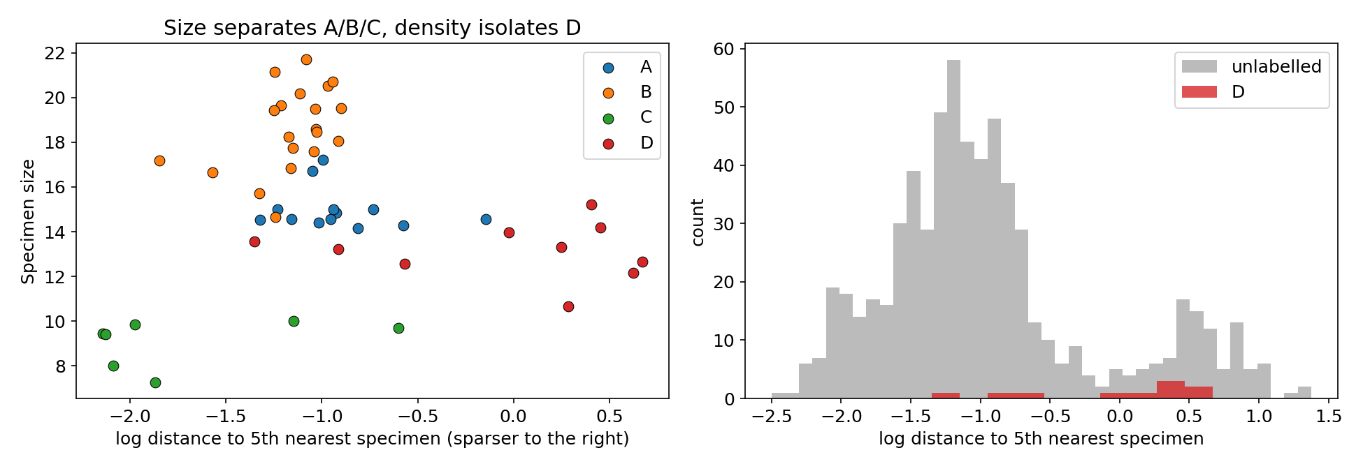
Left: labelled specimens in the (density, size) plane: size separates A, B and C, density isolates D. Right: the density feature of the 650 unlabelled specimens has two modes, a crowded one and a sparse one, and the labelled D fall in the sparse mode.

Two remarks explain why this works so well with only 50 labels.

It is semi-supervised for free: the 650 unlabelled specimens carry no strain, but they carry the shape of the terrain. Using them to measure density injects that knowledge into the classifier without touching their (unknown) labels. The test set is never used for it.
It respects the statement's rule "no cluster labels as features": we do not feed a cluster ID, we feed a continuous geometric quantity.

The same insight solves Q2: a density-based clustering finds the three terrains and declares the scattered specimens to be noise. DBSCAN on standardised $(X, Y)$ with $\varepsilon = 0.15$ and 5 neighbours gives exactly three clusters plus a noise group (right panel of the first figure), and reaches NMI 0.86. In Q2 the parameter $k$ is ignored by DBSCAN: the number of groups is a result, not an input, which is precisely what you want when one of the "groups" is background noise.

The full solution

Clustering (Q2). Standardise $(X, Y)$ , run DBSCAN ( $\varepsilon = 0.15$ , min_samples = 5). Evaluate against the 50 known strains: NMI 0.862, homogeneity 0.849, completeness 0.874. With k-means and $k = 4$ : NMI 0.500. The scan $\varepsilon \in \{0.15, 0.2, 0.25, 0.3\}$ gives 0.86, 0.79, 0.51, 0.43: as $\varepsilon$ grows, the arc and the line merge through the noise.
Features (Q3). $X$ , $Y$ , size, carnivore flag, and $\log d_5$ computed against the 700 training specimens (for a training point, its own entry is skipped; for a new specimen, the 5 nearest training specimens are used).
Model. Standardise the five features and fit a logistic regression on the 50 labelled rows. A linear model is a good fit for 50 examples: the classes are almost separable by thresholds on size and density.

nn = NearestNeighbors(n_neighbors=6).fit(train[["X", "Y"]])
dist, _ = nn.kneighbors(train[["X", "Y"]])
density = np.log(dist[:, 5])                 # column 0 is the specimen itself
X = np.c_[x, y, size, carnivore, density]
clf = LogisticRegression(max_iter=2000).fit(scaler.fit_transform(X[labelled]), strain[labelled])

Prediction (Q4). classify_unnown computes the same five features for one specimen and returns the predicted letter.

Results

Public test set: 50 fully labelled specimens (official labels). Cross-validation: 5-fold stratified, repeated 10 times, on the 50 labelled training specimens only.

approach	CV accuracy	public test accuracy
random forest on $(X, Y)$ only		0.72
random forest on size only		0.64
logistic regression, 4 raw features	0.83	0.78
random forest, 4 raw features	0.86	0.82
1-nearest neighbour, 4 raw features	0.88	0.86
label spreading over the 700 specimens (kNN graph)		0.76 to 0.86
random forest + density feature	0.87	0.90
logistic regression + density feature (final)	0.87 to 0.89	0.96

Confusion matrix of the final model on the public test (rows = truth A, B, C, D): A 18/18, B 12/12, C 7/7, D 11/13 (two D predicted B, both captured right next to the line).

clustering of $(X, Y)$	NMI	homogeneity	completeness
k-means, $k = 4$	0.500	0.497	0.503
DBSCAN, $\varepsilon = 0.15$	0.862	0.849	0.874

Honest caveats: with 50 test specimens, one error is worth 2 points of accuracy, and the cross-validation (on 50 labels) cannot distinguish the models with density from the best ones without it. The choice of the density feature was made from the exploration (D is scattered), not from the test score; the jump on the test (0.82 to 0.90 or 0.96) is consistent with the confusion matrices, where the errors on D are exactly what the feature fixes.

What to remember

Plot the map first. Two minutes of plotting showed arcs, lines, a blob and background noise, which dictated every later choice.
Match the clustering algorithm to the cluster shape. k-means wants round, comparable blobs and assigns every point; DBSCAN follows dense regions of any shape and is allowed to say "noise". The noise was a class here.
A class can be defined by density, not by position. When a class lives "everywhere sparse", give the model a neighbourhood feature such as the distance to the $k$ -th neighbour.
Unlabelled data still carries information. 650 unlabelled points told us where the terrains are; computing features against them is the simplest form of semi-supervised learning.
With 50 labels, prefer simple models and read the confusion matrix: it tells you which feature is missing far better than another round of hyperparameter tuning.

"""INAIO 2025 Stage 2, Problem 5: Classifying the Unnown.

Q2: location clusters with DBSCAN (the terrain is an arc, a line and a blob plus scattered noise).
Q3/Q4: a classifier on location + size + diet + a LOCAL DENSITY feature computed against ALL 700
training specimens (labelled or not): strain D lives in the sparse 'noise' between the dense
terrains, so 'how crowded is my neighbourhood' is the missing feature.
Usage: python solution.py data/unnown_train.csv data/unnown_test_public.csv
"""
import sys
import numpy as np, pandas as pd
from sklearn.cluster import KMeans, DBSCAN
from sklearn.linear_model import LogisticRegression
from sklearn.neighbors import NearestNeighbors
from sklearn.preprocessing import StandardScaler
from sklearn.metrics import (accuracy_score, confusion_matrix, normalized_mutual_info_score,
                             homogeneity_score, completeness_score)

K_DENS = 5  # density = distance to the 5th nearest specimen


# ---------------- Q2: location clusters ----------------
def learn_location_clusters(df: pd.DataFrame, k: int, method: str = "dbscan") -> pd.DataFrame:
    """Cluster on standardised (X, Y). DBSCAN ignores k: it finds the dense terrains itself and
    labels scattered specimens -1 (noise), which is exactly strain D."""
    Z = StandardScaler().fit_transform(df[["X", "Y"]])
    if method == "kmeans":
        df["Cluster_ID"] = KMeans(n_clusters=k, random_state=42, n_init=10).fit_predict(Z)
    else:
        df["Cluster_ID"] = DBSCAN(eps=0.15, min_samples=5).fit_predict(Z)
    return df


def cluster_metrics(path, k=4, method="dbscan"):
    df = learn_location_clusters(pd.read_csv(path), k, method)
    lab = df.dropna(subset=["Genetic_Label"])
    t, p = lab["Genetic_Label"], lab["Cluster_ID"]
    return {"NMI": normalized_mutual_info_score(t, p), "Homogeneity": homogeneity_score(t, p),
            "Completeness": completeness_score(t, p)}


# ---------------- Q3: classifier ----------------
def _base(df):
    return np.c_[df["X"], df["Y"], df["Specimen_Size"], (df["Diet_Type"] == "Carnivore").astype(float)]


def learn_unnown_classifier(train_file_path: str):
    df = pd.read_csv(train_file_path)
    # density reference = every training specimen, labelled or not (650 of 700 are unlabelled)
    nn = NearestNeighbors(n_neighbors=K_DENS + 1).fit(df[["X", "Y"]].values)
    dist, _ = nn.kneighbors(df[["X", "Y"]].values)
    dens = np.log(dist[:, K_DENS])                  # column 0 is the point itself
    X = np.c_[_base(df), dens]
    scaler = StandardScaler().fit(X)
    lab = df["Genetic_Label"].notna().values
    clf = LogisticRegression(max_iter=2000).fit(scaler.transform(X[lab]), df["Genetic_Label"][lab].astype(str))
    return {"nn": nn, "scaler": scaler, "clf": clf}


def classify_unnown(features: dict, model) -> str:
    xy = np.array([[features["X"], features["Y"]]])
    dist, _ = model["nn"].kneighbors(xy, n_neighbors=K_DENS)  # a new specimen is not in the pool
    row = pd.DataFrame([features])
    X = np.c_[_base(row), np.log(dist[:, K_DENS - 1])]
    return str(model["clf"].predict(model["scaler"].transform(X))[0])


if __name__ == "__main__":
    train_path, test_path = sys.argv[1], sys.argv[2]
    for m in ("kmeans", "dbscan"):
        print(m, {k: round(v, 3) for k, v in cluster_metrics(train_path, 4, m).items()})
    model = learn_unnown_classifier(train_path)
    te = pd.read_csv(test_path)
    feats = [c for c in te.columns if c not in ("Specimen_ID", "Genetic_Label")]
    pred = te[feats].apply(lambda r: classify_unnown(r.to_dict(), model), axis=1)
    print("public test accuracy", accuracy_score(te["Genetic_Label"], pred))
    print(confusion_matrix(te["Genetic_Label"], pred, labels=list("ABCD")))

Classifying the Unnown: Decoding the Mystery of Genetics and Terrain