IOAI Training: Learn AI by solving problems

The problem in brief

Researchers record signals from a space antenna. Each observation has a "primary signal" of 4 800 numbers and a 128-number "modulation signal" that describes how the antenna was configured. Every observation comes from one of four space objects, and you must say which one. There are 1 650 labelled training observations and 660 test observations. The statement hints that the 1-D signals hide a structure that "might be reconstructed into a more meaningful form", and that the modulation signal affects noise. This is a Kaggle simulation from the first training camp (Pelatnas 1) of Indonesia's IOAI 2026 team selection.

How you are scored

Plain classification accuracy on the test set:

\text{accuracy} = \frac{\#\{\text{correct predictions}\}}{\#\{\text{test observations}\}} .

The test labels and the Kaggle leaderboard require a login, so we report 5-fold stratified cross-validation accuracy on the training set and say clearly that the official test labels are private. The classes are imbalanced (700 / 500 / 300 / 150), so always predicting class 0 already gives 42.4 %.

First look at the data

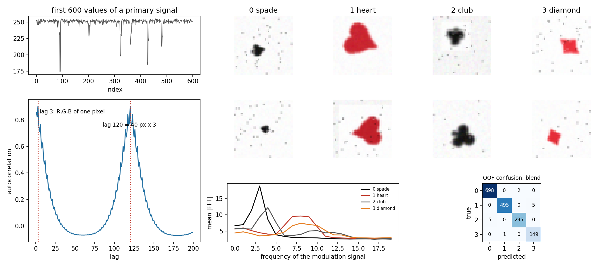
The primary signal is an image. Its values are integers from 1 to 255, like pixel intensities. The autocorrelation of the sequence has sharp peaks at lag 3 and at lag 120, a fingerprint of an image stored row by row with three colour channels: lag 3 jumps from one pixel's red value to the next pixel's red value, and lag 120 = 40 pixels x 3 channels jumps one row down. And $4800 = 40 \times 40 \times 3$ . Reshaped to $40 \times 40$ RGB, every observation shows a playing-card suit: class 0 is a spade, 1 a heart, 2 a club, 3 a diamond. The images are degraded by salt noise, blur, darker backgrounds, and random rotations, scales and positions.

The modulation signal carries class information in its frequency content. It does not explain the noise level: a ridge regression from the modulation signal to the salt-noise fraction, the background level or the blur gives $R^2 \approx 0$ . But its spectrum differs strongly between classes. Spades peak at frequency 3, clubs at 4, while hearts and diamonds have broad peaks around frequencies 7 to 10.

A first baseline

approach	5-fold CV accuracy
always predict class 0	0.424
two colour features (redness, dark-pixel count), gradient boosting	0.699
raw 1-D primary signal, PCA (100) + logistic regression	0.755
same after a 3x3 median filter	0.753
modulation signal as raw values, logistic regression	0.367
modulation signal as raw values, gradient boosting	0.786

Colour separates red suits from black ones but not a spade from a club. A linear model on raw pixels cannot cope with symbols that move, rotate and change size. A linear model on the raw modulation values fails, because the information is in the frequency, not in the values at fixed positions (a phase shift changes every value but not the spectrum).

The key idea

Rebuild the right representation of each signal, then use a model whose inductive bias matches it.

The primary signal is an image of a shape that can appear anywhere, at any rotation. A convolutional network has the right biases: local filters, weight sharing (translation invariance) and pooling. We add augmentation with the transformations present in the data (90-degree rotations, left-right mirrors, small shifts), and test-time augmentation (averaging the predictions over the four rotations). The salt noise is handled by the network itself; an explicit median filter did not help the linear baseline.
The modulation signal is a 1-D waveform whose class shows up in its dominant frequency. Its FFT magnitude is invariant to shifts in time and makes the class visible, so gradient boosting on the spectrum reaches about 91 % with no image at all.
The two views make mostly different mistakes. The CNN sometimes confuses spade and club (similar black shapes, small after blur) or heart and diamond, while the modulation spectrum separates spades from clubs well (peaks at 3 and 4). Adding their log-probabilities combines the evidence, as a naive-Bayes product of two experts would.

The full solution

Reshape each primary signal: values / 255, then reshape(40, 40, 3) and transpose to channels-first.
CNN: three blocks of (conv 3x3, BatchNorm, ReLU) x 2 + max-pool, with 32, 64 and 128 channels, then global average pooling, dropout 0.3 and a linear layer to 4 classes. Class-weighted cross-entropy (for the imbalance), AdamW and a one-cycle learning-rate schedule, 30 epochs with batch size 64 on Apple MPS, random rotation, mirror and shift at each batch.
Modulation: np.abs(np.fft.rfft(m)), then HistGradientBoostingClassifier with balanced class weights.
Blend: $\log p = 0.9 \log p_{\text{CNN}} + 0.1 \log p_{\text{mod}}$ , with the weight chosen on out-of-fold predictions, then argmax.

def augment(x):
    x = torch.rot90(x, np.random.randint(4), (2, 3))      # suits appear rotated
    if np.random.rand() < .5: x = torch.flip(x, (3,))     # a mirrored suit keeps its identity
    dx, dy = np.random.randint(-3, 4, 2)
    return torch.roll(x, (int(dx), int(dy)), (2, 3))

The final model, trained on all 1 650 observations, predicts test classes in proportions 280 / 200 / 120 / 60. These are exactly the training proportions scaled to 660 rows, a good sign that the test set was drawn the same way.

Results

5-fold stratified cross-validation (official test labels are private):

approach	CV accuracy
majority class	0.424
colour features + gradient boosting	0.699
raw signal, PCA + logistic regression	0.755
median filter + PCA + logistic regression	0.753
median filter + modulation, PCA + logistic regression	0.739
modulation raw values, gradient boosting	0.786
modulation spectrum, gradient boosting	0.915
CNN on reshaped images, no augmentation	0.955
CNN + augmentation	0.967
CNN + augmentation + test-time augmentation (4 rotations)	0.979
blend CNN + modulation spectrum (final)	0.992

The blend makes 13 errors out of 1 650: 5 hearts predicted as diamonds, 5 clubs as spades, 2 spades as clubs, and 1 diamond as a heart. The single blend weight was picked on the same out-of-fold predictions, so 0.992 is very slightly optimistic. The gain over the CNN alone (36 errors) is far larger than this selection effect.

What to remember

Look at the raw numbers and their autocorrelation. Values from 1 to 255, peaks at lags 3 and 40 x 3, and $4800 = 40 \times 40 \times 3$ revealed that the "1-D signal" was an RGB image.
Choose the representation before the model: images go to a CNN with augmentation matching the variations in the data, and waveforms go through an FFT when the information lives in frequencies.
Test what an auxiliary input really encodes. The modulation signal was described as an antenna setting linked to noise, but it predicted nothing about noise and a lot about the class.
Blend complementary views: two models with different error patterns, combined in log-probability space, beat either one by a wide margin.
Use class weights for imbalanced classes, and check the predicted class proportions on the test set as a sanity check.

"""Complicated Outer-Space Signals (Pelatnas 1 IOAI 2026, simulation 2, Indonesia).

Key idea: the 4800-value "primary signal" is a flattened 40x40 RGB image (lag-3 and lag-120 autocorrelation),
showing a playing-card suit (0 spade, 1 heart, 2 club, 3 diamond) with salt noise, blur, rotation and scale.
The 128-value "modulation signal" carries class information in its spectrum (dominant frequency).
Pipeline: (1) reshape to images, small CNN with rotation/flip/shift augmentation;
          (2) gradient boosting on the modulation spectrum;
          (3) blend the two probability vectors (weight chosen on out-of-fold predictions).
Data: multimodal_train.csv and multimodal_test_data.csv in ./ (Drive zip of the task).
"""
import os
os.environ.setdefault("OMP_NUM_THREADS", "2")
import numpy as np, pandas as pd, torch, torch.nn as nn, torch.nn.functional as F
from sklearn.model_selection import StratifiedKFold
from sklearn.ensemble import HistGradientBoostingClassifier

torch.set_num_threads(2); torch.manual_seed(0); np.random.seed(0)
dev = "mps" if torch.backends.mps.is_available() else "cpu"

tr = pd.read_csv("multimodal_train.csv"); te = pd.read_csv("multimodal_test_data.csv")
y = tr["label"].values
P_COLS = [f"primary_{i}" for i in range(4800)]; M_COLS = [f"modulation_{i}" for i in range(128)]
to_img = lambda df: np.ascontiguousarray((df[P_COLS].values / 255.0).reshape(-1, 40, 40, 3).transpose(0, 3, 1, 2))
Xi, Xi_te = torch.tensor(to_img(tr), dtype=torch.float32), torch.tensor(to_img(te), dtype=torch.float32)
spec = lambda df: np.abs(np.fft.rfft(df[M_COLS].values, axis=1))      # modulation -> magnitude spectrum
S, S_te = spec(tr), spec(te)

class Net(nn.Module):
    def __init__(s):
        super().__init__()
        def blk(i, o): return nn.Sequential(nn.Conv2d(i, o, 3, padding=1), nn.BatchNorm2d(o), nn.ReLU(),
                                            nn.Conv2d(o, o, 3, padding=1), nn.BatchNorm2d(o), nn.ReLU(), nn.MaxPool2d(2))
        s.net = nn.Sequential(blk(3, 32), blk(32, 64), blk(64, 128), nn.AdaptiveAvgPool2d(1), nn.Flatten(),
                              nn.Dropout(0.3), nn.Linear(128, 4))
    def forward(s, x): return s.net(x)

def augment(x):
    # the suits appear rotated, mirrored and shifted: teach the CNN these invariances
    x = torch.rot90(x, np.random.randint(4), (2, 3))
    if np.random.rand() < .5: x = torch.flip(x, (3,))
    dx, dy = np.random.randint(-3, 4, 2)
    return torch.roll(x, (int(dx), int(dy)), (2, 3)).contiguous()

def train_cnn(idx, epochs=30):
    net = Net().to(dev); opt = torch.optim.AdamW(net.parameters(), 2e-3, weight_decay=1e-4)
    sched = torch.optim.lr_scheduler.OneCycleLR(opt, 3e-3, total_steps=epochs * (len(idx) // 64 + 1))
    w = torch.tensor(len(idx) / (4 * np.bincount(y[idx])), dtype=torch.float32, device=dev)   # imbalance
    Y = torch.tensor(y)
    for _ in range(epochs):
        net.train(); perm = np.random.permutation(idx)
        for b in range(0, len(perm), 64):
            i = perm[b:b + 64]
            loss = F.cross_entropy(net(augment(Xi[i]).to(dev)), Y[i].to(dev), weight=w)
            opt.zero_grad(); loss.backward(); opt.step(); sched.step()
    return net

@torch.no_grad()
def cnn_proba(net, X):
    # test-time augmentation: average over the 4 rotations
    net.eval()
    return np.mean([F.softmax(net(torch.rot90(X, k, (2, 3)).contiguous().to(dev)), 1).cpu().numpy() for k in range(4)], 0)

hgb = lambda: HistGradientBoostingClassifier(max_iter=300, learning_rate=0.05, class_weight="balanced", random_state=0)

# ---------- out-of-fold predictions (honest validation: official test labels are private)
oof_c, oof_m = np.zeros((len(y), 4)), np.zeros((len(y), 4))
for f, (a, b) in enumerate(StratifiedKFold(5, shuffle=True, random_state=0).split(S, y)):
    oof_c[b] = cnn_proba(train_cnn(a), Xi[b])
    oof_m[b] = hgb().fit(S[a], y[a]).predict_proba(S[b])
    print(f"fold {f}: CNN {np.mean(oof_c[b].argmax(1) == y[b]):.4f}  modulation {np.mean(oof_m[b].argmax(1) == y[b]):.4f}", flush=True)
acc = lambda p: np.mean(p.argmax(1) == y)
print(f"OOF accuracy  CNN+TTA {acc(oof_c):.4f} | modulation spectrum HGB {acc(oof_m):.4f}")
ws = np.linspace(0, 1, 21)
scores = [acc(np.log(oof_c + 1e-9) * (1 - w) + np.log(oof_m + 1e-9) * w) for w in ws]
w_best = ws[int(np.argmax(scores))]
print(f"blend (log-prob) weight on modulation {w_best:.2f}: OOF accuracy {max(scores):.4f}")
np.save("oof.npy", np.stack([oof_c, oof_m]))

# ---------- final models on all training data, predict the test set
net = train_cnn(np.arange(len(y)))
p = np.log(cnn_proba(net, Xi_te) + 1e-9) * (1 - w_best) + np.log(hgb().fit(S, y).predict_proba(S_te) + 1e-9) * w_best
pd.DataFrame({"id": np.arange(len(te)), "label": p.argmax(1)}).to_csv("submission.csv", index=False)
print("submission.csv written, predicted class counts:", np.bincount(p.argmax(1), minlength=4))