Essay Paper

The problem in brief

This is the written paper of the 2025 Indonesian IOAI selection exhibition round. It has seven independent exercises, in Indonesian: a logic puzzle (two robots locating a star on a 6 by 6 board), reading a rule-based decision plot, gradient descent on the squared hinge loss, bigram probabilities, hand-made features for 5 by 5 binary images, choosing a metric for a rare disease, and eigenvectors with diagonalisation. Every answer below is derived from scratch and checked numerically by solution.py. No official answer key is published. Exercise 5 prints a "Key" label for each test image, and we compare our rule with it.

How you are scored

The paper is marked by hand, exercise by exercise, with partial credit for correct reasoning. Exercise 1 explicitly gives partial credit for eliminating some of the stars, even without the final answer. No points table or pass mark is published.

The full solution

1. The two robots and Aoi's star

The stars sit at C1, E1, B2, D2, A3, E3, B4, D4, F4, C5, A6, D6, F6. ROBOBAR knows the row, ROBOKOL knows the column, and each line of the dialogue is public, so both robots (and we) can delete candidates as they go.

The rule for "I don't know": a robot that knows the row would know the star if its row contained a single remaining candidate. So "I don't know" from ROBOBAR deletes every candidate that is alone in its row, and the same from ROBOKOL deletes every candidate alone in its column.

1. ROBOBAR, "I don't know". Row 5 has a single star, so C5 goes.
2. ROBOKOL, "I don't know". Column C now holds only C1, so C1 goes.
3. ROBOBAR, "I don't know". Row 1 now holds only E1, so E1 goes.
4. ROBOKOL, "I don't know". Column E now holds only E3, so E3 goes.

That leaves B2, D2, A3, B4, D4, F4, A6, D6, F6.

5. ROBOBAR, "we could go on forever". Imagine the dialogue going on. Row 3 now has only A3, so a further "I don't know" would delete it. Then column A has only A6, which goes next. After that, no row or column holds a single candidate any more. The stuck set, where the conversation really would go on forever, is therefore $S=\{B2, D2, B4, D4, F4, D6, F6\}$. ROBOBAR can only claim "forever" if every candidate in his row lies in $S$. Row 6 contains A6, which would eventually be found. If his row were 3, he would already know. So his row is 2 or 4, and the candidates become B2, D2, B4, D4, F4.
6. ROBOKOL, "now I know". Column B holds B2 and B4, and column D holds D2 and D4, so in either case he could not decide. Column F holds only F4.

Aoi's star is F4.

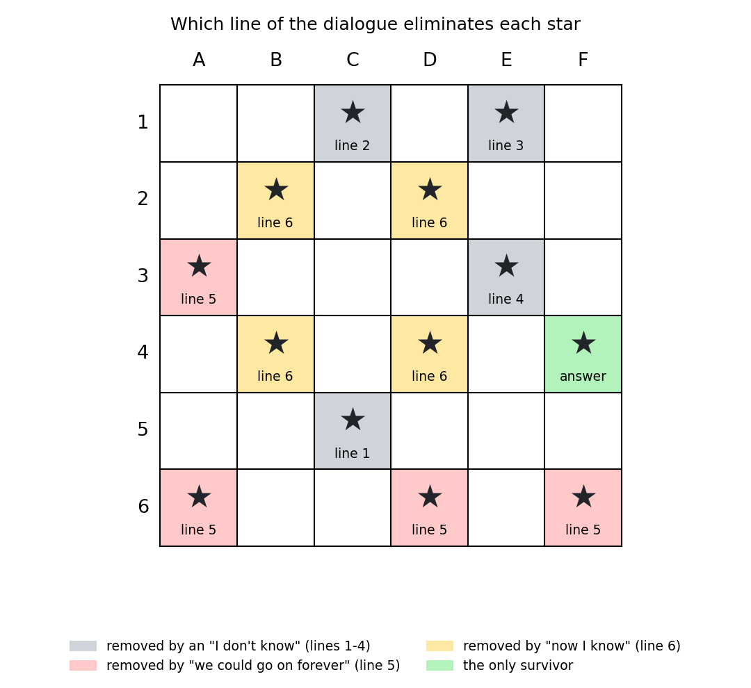
The pattern to remember: each public statement of ignorance is information. The "forever" statement is a statement about a fixed point of the elimination process, so you have to run that process to its end.

2. Decision plot

Measuring the figure's pixels (the colour changes fall exactly on the grid lines at 2, 6 and 8) gives these rules:

• if $x_1 < 6$: class 0 when $x_2 < 8$, class 2 otherwise;
• if $x_1 \ge 6$: class 0 when $x_2 < 2$, class 1 when $2 \le x_2 < 6$, class 2 when $x_2 \ge 6$.

1. $(8, 3)$ has $x_1 \ge 6$ and $2 \le 3 < 6$, so it is class 1.

2. Classes 1 and 2 are separated by $x_2 = 6.00$ (for $x_1 \ge 6$).

3. Applying the rules to the 8 points: $(5.86, 3.62)$, $(0.53, 6.51)$, $(5.69, 7.46)$, $(2.53, 1.52)$ and $(6.42, 0.85)$ are class 0. $(9.50, 5.93)$ and $(9.29, 4.36)$ are class 1. $(6.28, 6.20)$ is class 2. So (a) 5, (b) 2, (c) 1. Watch $(6.42, 0.85)$: $x_1 \ge 6$, but it falls in the blue strip under $x_2 = 2$.

4. For a uniform point, probability is area divided by 100:

   • class 0 covers $6\times 8 + 4\times 2 = 56$, so 0.56;
   • class 1 covers $4\times 4 = 16$, so 0.16;
   • class 2 covers $6\times 2 + 4\times 4 = 28$, so 0.28.

   They add up to 1, as they must.

3. Squared hinge loss

With $f(x)=wx+b$ and margin deficit $m_i=\max\{0,\,1-y_i f(x_i)\}$, the loss is $L=\frac15\sum_i m_i^2$.

Q1. At $w=b=0$, every $m_i = 1$, so $L=1$.

Q2. Where $m_i>0$, $\partial m_i/\partial w = -y_i x_i$ and $\partial m_i/\partial b = -y_i$. Where $m_i=0$, the term is flat. At the kink $m_i = 0$ both one-sided derivatives of $m_i^2$ are 0, so the squared hinge is differentiable everywhere. That is its advantage over the plain hinge. Hence:

$$\frac{\partial L}{\partial w} = -\frac{2}{5}\sum_{i=1}^{5} m_i\, y_i\, x_i , \qquad \frac{\partial L}{\partial b} = -\frac{2}{5}\sum_{i=1}^{5} m_i\, y_i .$$

Q3. At the origin, all $m_i=1$. We have $\sum y_i x_i = -2.1+0.7-0.2-0.8+2.2=-0.2$ and $\sum y_i = -1$, so

$$\frac{\partial L}{\partial w} = 0.08, \qquad \frac{\partial L}{\partial b} = 0.4 ,$$

and one step with $\eta=1$ gives $w=-0.08$, $b=-0.4$. The new margins $1-y_if(x_i)$ are $1.232, 0.656, 0.584, 0.536, 1.576$, so $L = 5.0603/5 \approx 1.0121$. The loss went up: $\eta = 1$ is too large for this problem. A second step gives $L\approx1.142$, and if you keep going, the iterates diverge.

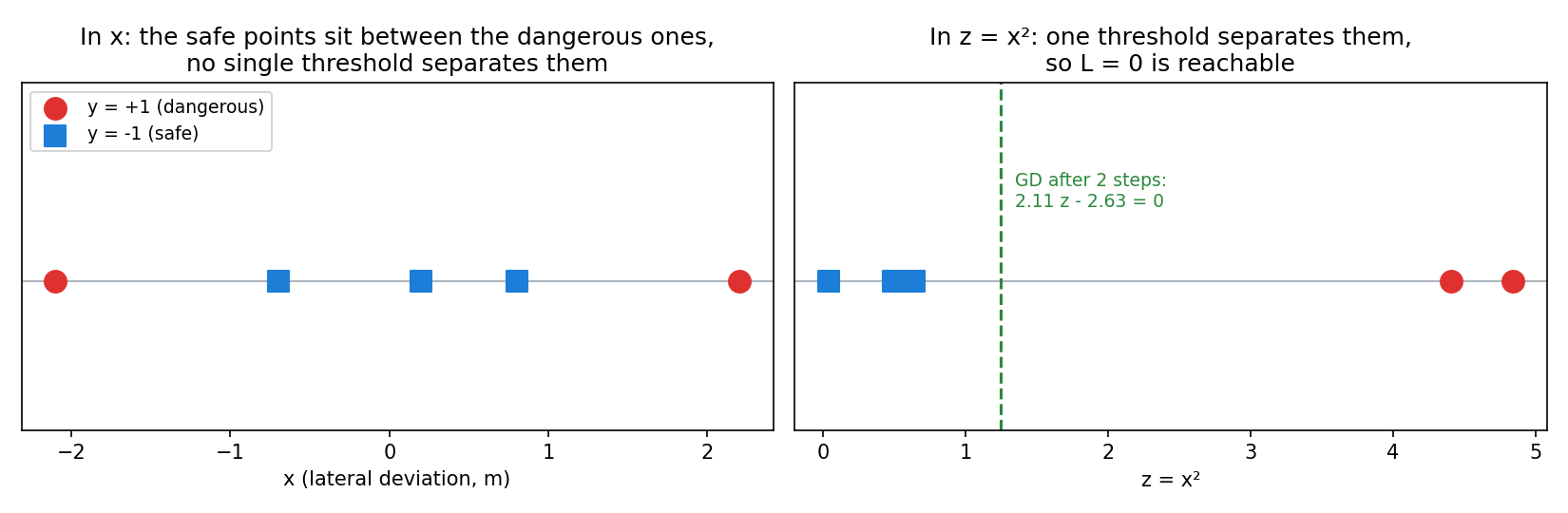
Q4. No. $L=0$ would need $f(-2.1)\ge 1$ and $f(2.2) \ge 1$ but $f(0.2)\le -1$. A linear $f$ evaluated at $0.2$, which lies between $-2.1$ and $2.2$, is a convex combination of the two end values, so it is at least 1. Contradiction. The dangerous cars are on both sides of the safe ones, so no single threshold on $x$ separates them. The best achievable loss, with a small learning rate, is about $0.960$. Gradient descent can at best converge to that minimum, never to 0.

Q5. Yes. With $z=x^2$, the dangerous points have $z\in\{4.41, 4.84\}$ and the safe ones $z\in\{0.49, 0.04, 0.64\}$. These are separated by a threshold, with room for margin 1. For example, $w=1$ and $b=-2.5$ give $y_if\ge1.86$ for every point. Squaring the feature turned a two-sided rule ("too far left OR too far right") into a one-sided one.

Q6. On $z$, with $\eta = 1$:

• $t=1$: $\sum y_i z_i = 8.08$, so $\partial L/\partial w=-3.232$ and $\partial L/\partial b=0.4$. This gives $w^{(1)}=3.232$, $b^{(1)}=-0.4$ and $L^{(1)}\approx 2.4842$. The two dangerous points now have margin above 1, but the safe ones are pushed to the wrong side.
• $t=2$: only the three safe points still contribute. $\partial L/\partial w = 0.4\,(2.1837\cdot0.49+0.7293\cdot0.04+2.6685\cdot0.64)=1.1228$ and $\partial L/\partial b = 0.4\,(2.1837+0.7293+2.6685)=2.2326$. This gives $w^{(2)}\approx 2.1092$, $b^{(2)}\approx-2.6326$ and $L^{(2)} = 0$: every point now has $y_i f \ge 1$. For instance $z=0.64$ gives $f=-1.28$, and $z=4.41$ gives $f=6.67$.

4. Probability (bigrams)

Both first words were seen in 100 sentences, so they are equally likely a priori, and Bayes reduces to a ratio of counts.

1. (a) $P(\text{lura}\mid\text{domi}) = \dfrac{48}{48+42} = \dfrac{8}{15} \approx 0.533$. (b) $P(\text{kira}\mid\text{salu}) = \dfrac{25}{27+25} = \dfrac{25}{52}\approx 0.481$.
2. The 10 sentences are independent, and each has first word "lura" with probability $p = 8/15$, so the count is binomial:

$$P(X=6) = \binom{10}{6} \left(\tfrac{8}{15}\right)^{6} \left(\tfrac{7}{15}\right)^{4} \approx 0.229 .$$

5. Feature extraction

$A_1$ is a pattern of stripes (columns all 1 or all 0). $A_2$ is a checkerboard. Allowed distortions are rotation, shift and noise. A rotation by 90 degrees turns vertical stripes into horizontal ones and leaves a checkerboard unchanged. A one-pixel shift swaps the phase. So each class is a small family of perfect patterns: 4 stripe patterns (vertical or horizontal, 2 phases each) and 2 checkerboards.

Features (Q2).

• $d_{\text{stripes}}$ is the smallest number of pixels that differ from one of the 4 perfect stripe patterns.
• $d_{\text{checker}}$ is the same count for the 2 checkerboards.

Both are computed directly from the entries, e.g. $\sum_{i,j}\lvert M_{ij} - [\,(j+p) \bmod 2 = 0\,]\rvert$. They generalise the statement's example feature "full column of ones": a perfect $A_1$ has $d_{\text{stripes}}=0$ because its columns are uniform.

image	$d_{\text{stripes}}$	$d_{\text{checker}}$	nearest pattern	rule $d_{\text{stripes}}\le4$	printed key
T1	0	10	A1	A1	A1
T2	0	10	A1	A1	A1
T3	4	6	A1	A1	A1
T4	6	4	A2	A2	A2
T5	7	5	A2	A2	A2
T6	10	0	A2	A2	A2
T7	3	11	A1	A1	A1
T8	6	12	A1	A2	A2
T9	2	8	A1	A1	A1
T10	6	12	A1	A2	A2

Decision rule (Q1 and Q3). The natural rule, "pick the class whose nearest perfect pattern is closer", reproduces 8 of the 10 printed keys. T8 and T10 disagree with the key: both are 6 flips from horizontal stripes but 12 from any checkerboard, so the stated generation process (rotation + shift + noise) makes A1 the more plausible origin. The single rule that reproduces all ten printed keys is

$$\text{label}(T) = \begin{cases} A_1 & \text{if } d_{\text{stripes}}(T) \le 4,\\ A_2 & \text{otherwise,}\end{cases}$$

meaning: call it stripes only if at most 4 of the 25 pixels (16 %) break a stripe pattern. Because the threshold 4 was read off the keys themselves, we present it as the rule consistent with the answer sheet, and the nearest-pattern rule as the more principled one. T3 is worth a look: it is $A_1$ with rows 2 and 4 painted white. Painting the same rows white on $A_2$ gives exactly the same image, so T3 is ambiguous by construction. Only noise counts (4 versus 6 flips) favour A1.

6. Confusion matrix: choosing the metric

With 10 sick patients out of 1000, a system that always answers "healthy" scores 99 % accuracy while missing every patient, so accuracy is useless here. The two errors map onto two metrics:

• a missed diagnosis is a false negative, which lowers recall $= TP/(TP+FN)$;
• a false alarm is a false positive, which lowers precision $= TP/(TP+FP)$.

To weigh both in a balanced way, use the F1-score of the positive (sick) class:

$$F_1 = \frac{2PR}{P+R} = \frac{2\,TP}{2\,TP + FP + FN} .$$

The second form shows the point: F1 counts FP and FN symmetrically and ignores the 990 true negatives that make accuracy look good. The harmonic mean is high only if both precision and recall are high. F1-micro is not the right choice: in binary classification it equals accuracy. F1-macro is not either: it averages in the F1 of the healthy class, which is close to 1 for any model and hides the failures. In practice you would also choose the decision threshold on a validation set, and use $F_\beta$ with $\beta>1$ if the hospital later decides that misses are worse than false alarms.

7. Matrices

Q1. For $A=\begin{pmatrix}1&2\\5&4\end{pmatrix}$:

$$\det(A-\lambda I) = (1-\lambda)(4-\lambda)-10 = \lambda^2-5\lambda-6 = (\lambda-6)(\lambda+1).$$

• $\lambda_1=6$: the first row of $A - 6I$ gives $-5v_1+2v_2=0$, so $v=(2,5)^\top$ (any nonzero multiple). Check: $A(2,5)^\top = (12,30)^\top = 6\,(2,5)^\top$.
• $\lambda_2=-1$: $2v_1+2v_2=0$, so $v=(1,-1)^\top$. Check: $A(1,-1)^\top=(-1,1)^\top$.

Q2. Suppose $A=PDP^{-1}$ with $D=\operatorname{diag}(d_1,d_2)$ and $P$ invertible. Multiply on the right by $P$: $AP=PD$. Write $P=[\,p_1\ p_2\,]$ by columns. The $j$-th column of $AP$ is $Ap_j$. The $j$-th column of $PD$ is $P$ times the $j$-th column of $D$, that is $P(d_j e_j)=d_j p_j$. Hence

$$A p_1 = d_1 p_1, \qquad A p_2 = d_2 p_2 .$$

Since $P$ is invertible, its columns are nonzero (a zero column would make $\det P=0$). So each $p_j$ is an eigenvector of $A$ with eigenvalue $d_j$. In coordinates, the first column reads $a_{11}p_{11}+a_{12}p_{21} = d_1 p_{11}$ and $a_{21}p_{11}+a_{22}p_{21} = d_1 p_{21}$, and the same holds for the second column. With the example of Q1: $P=\begin{pmatrix}2&1\\5&-1\end{pmatrix}$ and $D=\operatorname{diag}(6,-1)$ satisfy $A=PDP^{-1}$.

Results

exercise	answer
1. Logic	the star is at F4
2. Decision plot	class 1; boundary $x_2=6.00$; counts 5 / 2 / 1; probabilities 0.56 / 0.16 / 0.28
3. Squared hinge	$L(0,0)=1$; step to $(-0.08,-0.4)$ with $L\approx1.0121$; $L=0$ impossible on $x$ (best 0.960); possible on $z=x^2$; $(3.232,-0.4)$ with $L\approx2.4842$, then $(2.1092,-2.6326)$ with $L=0$
4. Probability	$8/15\approx0.533$; $25/52\approx0.481$; $0.229$
5. Features	nearest-pattern rule: 8 of 10 printed keys (T8, T10 differ); rule $d_{\text{stripes}}\le4$ matches all 10
6. Metric	F1-score of the positive class
7. Matrices	$\lambda=6$ with $(2,5)$, $\lambda=-1$ with $(1,-1)$; proof via $AP=PD$

What to remember

• Statements of ignorance carry information, and "forever" means "in the fixed point of the elimination". Run the process to the end before reasoning about it.
• A feature map can make a problem linearly separable. On $x$, the two-sided rule "too far left or too far right" defeats any linear model. On $x^2$, one threshold is enough, and that is the idea behind kernels.
• Gradient descent is not guaranteed to decrease the loss. With $\eta=1$, the very first step increased it. Always check the loss after a step.
• On rare classes, use F1 (or precision and recall), not accuracy. F1 equals $2TP/(2TP+FP+FN)$: it treats both errors alike and ignores the many easy negatives.
• Hand-made features should encode the invariances you are told about (here rotation and shift). When a rule is tuned to match a given answer key, say so, and keep the principled version next to it.