Where Is Spy-C?

The problem in brief

A secret "Spies Group" of five animals (a beaver, a fox, a pigeon, a rabbit and a raccoon) is plotting to take over the world chocolate market. You are given 2 000 past missions, each described by 12 columns (where the agent last met an informant, where a radio signal was intercepted, the mission type, the agent's status, speciality and language level, contact frequency, duration, budget and a discretion score), together with the agent who carried it out. For 1 000 new missions you must do two things: name the agent from the table, and point to that agent in the mission's surveillance picture, a crowded "Where's Wally?" style drawing of 1024, 2048 or 4096 pixels. Every picture contains several animals, and the agent is the one wearing its own distinctive accessories: an orange hard hat and bow tie for the beaver, black sunglasses and a scarf for the fox, a fedora and a messenger bag for the pigeon, red sneakers and a backpack for the rabbit, a grey hoodie and round glasses for the raccoon. You get no annotated image at all, only five "off-duty" sprites of each animal without its accessories.

Data: the Kaggle dataset timmor/ofia2026 (tables and sprites) and the Hugging Face dataset OlympiadesIA/OFIA2026 (the 1 000 test images, 10.9 GB). The statement and the scoring rules come from the competition pages on Kaggle. The official test labels are private, and we never submitted anything. Identification is scored on a held-out split of the training table. For localisation, we ran our detector on a subset of 63 test images (every 16th one) and checked each predicted point by eye. The localisation number is therefore a self-made estimate, not an official score.

How you are scored

The score is out of 100, half for each part:

$$\text{Score} = 50\cdot\frac{\#\{\text{correct identities}\}}{1000} + 50\cdot\frac{\#\{\text{correct locations}\}}{1000}.$$

A location counts as correct when the predicted point falls in the $200\times200$ square around the agent's centre:

$$\max\big(|x-x^\ast|,\ |y-y^\ast|\big) \le 100 \text{ pixels}.$$

The two parts are linked. You must point to the animal of the true class, so a wrong identity almost always costs the location as well. If $a$ is the identification accuracy and $d$ is the probability of finding the right animal once you know who to look for, then roughly

$$\text{Score} \approx 50\,a + 50\,a\,d .$$

What to aim for. The organisers publish no threshold: the 100 best scores on the private leaderboard qualify. The competition leaderboard (read through the Kaggle API) is topped by 95.08, then 94.05 and 93.53. The organisers' example submission (random guesses) scores about 10.

First look at the data

The table. There are 2 000 training missions, exactly 400 per agent, and nothing is missing. Taken one at a time, the columns look almost useless: the class means of the contact frequency, budget and so on differ only a little, and the categorical columns are only mildly unbalanced. Then you plot the coordinates:

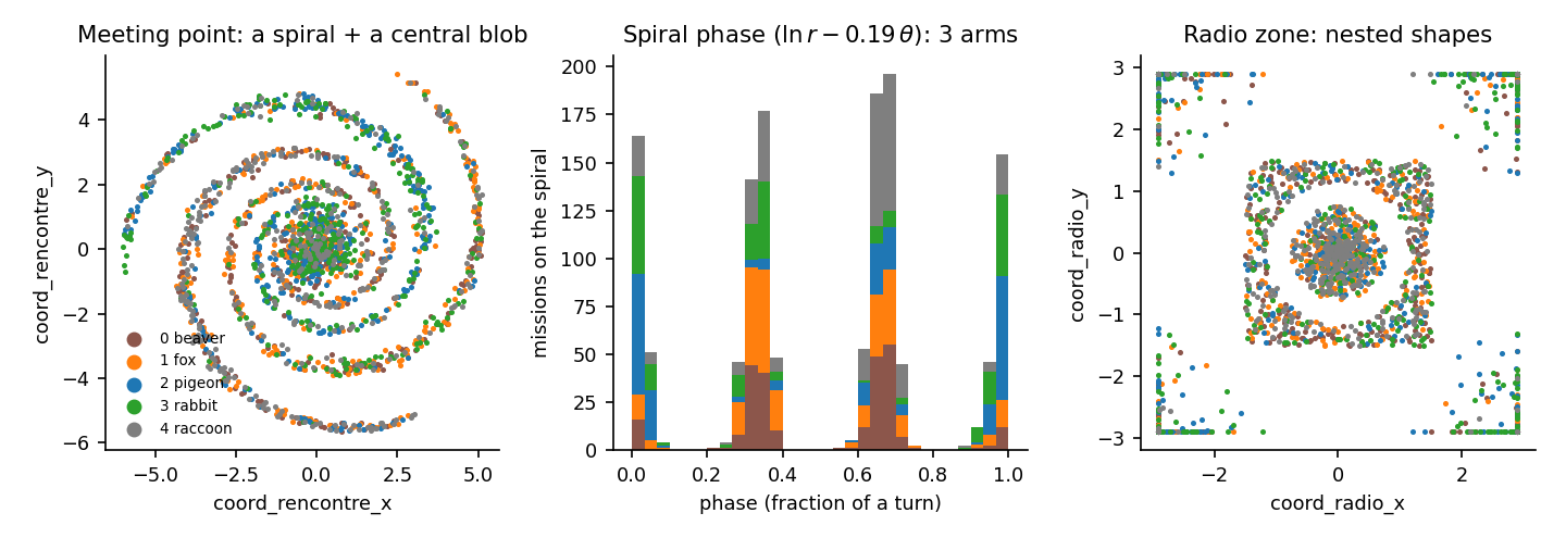
• The meeting point lies either on a logarithmic spiral (two thirds of the missions) or in a blob at the centre. In log-polar coordinates a log spiral $r = a\,e^{b\theta}$ becomes a straight line, since $\ln r = \ln a + b\theta$. So the quantity $(\ln r - b\theta)$, taken modulo one turn $2\pi b$, tells you which arm a point sits on. Scanning $b$ and keeping the value that makes this "phase" sharpest gives $b \approx 0.19$, and the histogram (middle panel) shows three arms. The arms are not shared equally: arm 0 is mostly the pigeon and the rabbit, while arms 1 and 2 hold the beaver, the fox and the raccoon.
• The radio zone lies in one of three nested shapes: a small disk, a square ring, and an outer frame squashed against the $\pm 2.9$ border. Here the raccoon and the fox favour the disk, while the pigeon and the rabbit favour the outer frame.

None of this can be read from $x$ and $y$ separately: a tree splitting on raw coordinates has to approximate a spiral with a staircase of rectangles. The structure only appears once you change coordinates.

The images. They are AI-generated cartoon scenes (a farm fair, a pirate harbour, a museum...) full of people, plus usually several of the five animals. The catch, which you only discover by looking at many images:

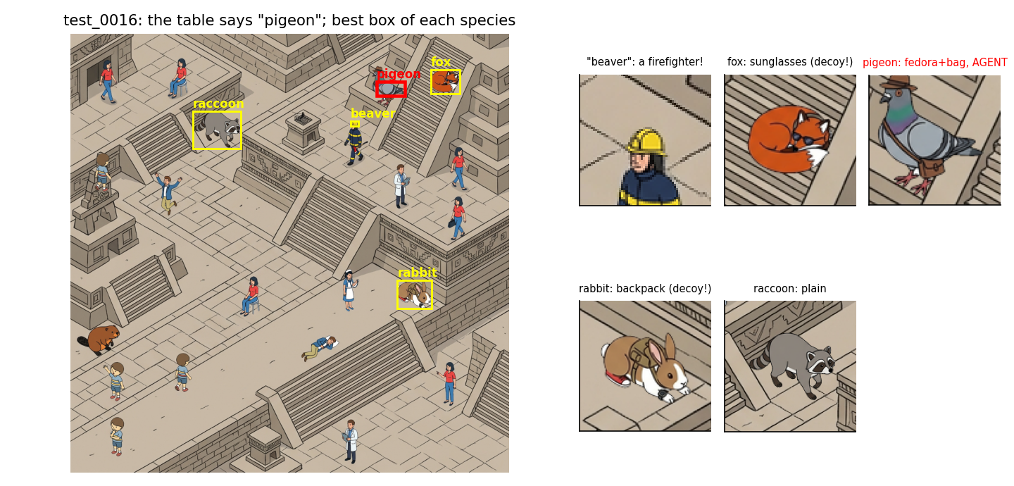
In test_0016, the table says "pigeon", and indeed the pigeon wears its fedora and bag. But the fox also wears sunglasses and the rabbit carries a backpack. Decoys wear accessories too, sometimes a full set. So the image does not reveal who the agent is: the table is needed for identity, and the image only for location. Notice also the pitfall in the figure: CLIP's best "beaver" is a firefighter in a yellow helmet. The real beaver, bottom left, wears nothing and is not the agent anyway.

A first baseline

Identity. On raw columns, 5-fold cross-validated accuracy is 0.30 for logistic regression, 0.50 for a random forest and 0.55 for gradient-boosted trees. That would give about 27 points out of 50.

Location. Without labelled images, the honest baseline is the image centre. That is almost never within 100 pixels of the agent, so it scores close to 0 out of 50.

The key idea

Two changes of viewpoint unlock the problem: polar coordinates for the table, and zero-shot vision models for the images.

1. Features that match how the data was generated. The class depends on which spiral arm and which radio shape a mission falls in, and these are simple functions of polar quantities:

$$r=\sqrt{x^2+y^2},\qquad \theta=\operatorname{atan2}(y,x),\qquad \text{phase} = \frac{(\ln r - b\,\theta) \bmod 2\pi b}{2\pi b},$$

and, for the radio zone, both the Euclidean radius and the "square radius" $\max(|x|,|y|)$, which tells a disk from a square ring. Each of these alone lifts boosting from 0.55 to between 0.60 and 0.68 (the spiral phase is the best single one). Together they reach 0.85, because the remaining columns (budget, duration, discretion score...) only become informative inside a given arm or shape. One example: the sign of score_discretion separates the beaver from the pigeon in the outer radio frame. That is again an interaction, which is why trees work here and Gaussian models (QDA, 0.29 to 0.51) do not.

2. Locating without training data. You cannot train a detector without boxes, but you can use models that already understand images and text. OWLv2 is an open-vocabulary detector: give it the text "a beaver" and it returns boxes. CLIP scores how well a crop matches a sentence. Our pipeline:

• Run OWLv2 with 11 text queries ("a beaver", ..., "a raccoon wearing a grey hoodie and round glasses", "an animal") on overlapping $1024\times1024$ tiles (4096 images are first halved). Merge the boxes with non-maximum suppression and keep the 40 best proposals.
• Crop each proposal with some margin and let CLIP compare it with 27 prompts: "a cartoon drawing of a beaver", the same with accessories, and 17 distractors ("a person", "a child", "a cow", "a barrel"...). The distractors matter: without "a person", the yellow-helmeted firefighter would become a very convincing beaver.
• For the agent $s$ predicted from the table, return the centre of the crop with the highest $P(s) + P(s \text{ with accessories})$.

Why not simply ask OWLv2 for "a beaver"? On whole images its species labels were unreliable: in test_0000 its best "beaver" box was the raccoon, and its best "rabbit" box was the beaver. OWLv2 is good at finding things that look like animals, while CLIP, looking at a crop enlarged to $224\times224$, is much better at telling which animal it is. Splitting "where" and "what" between two models is a classic zero-shot pattern.

The full solution

1. Identity. Drop the four raw coordinates and add: radius, angle and square radius for both points, the spiral phase with $b = 0.19$, the arm index (0, 1, 2, or "centre"), and the position along the arm $(\ln r - c_{\text{arm}})/b$. Then fit HistGradientBoostingClassifier with 300 rounds, learning rate 0.05 and 31 leaves:

ph = np.mod(np.log(r) - SPIRAL_B * theta, PER) / PER          # PER = 2*pi*b: one turn
D["arm"] = np.where(r < 1.8, -1, np.round(ph * 3) % 3)          # 3 arms, or the centre blob
D["phi"] = np.where(D.arm >= 0, (np.log(r) - D.arm / 3 * PER) / SPIRAL_B, -10)

2. Location. OWLv2 (google/owlv2-base-patch16-ensemble) proposals on tiles, then CLIP ViT-B/16 classification of the crops, as described above. On 2 CPU threads this takes about 7 s for a 1024 image and 30 to 40 s for a 2048 or 4096 image (about 20 minutes for our 63-image subset, and roughly 6 hours for all 1 000).

3. Submission. One row per mission: the predicted identity, and the centre of the chosen crop in original pixels.

Results

Identification (5-fold CV on the 2 000 training missions, plus a held-out 20 % split):

approach	accuracy	points / 50
logistic regression, raw columns	0.299	15.0
random forest, raw columns	0.502	25.1
gradient boosting, raw columns	0.550	27.5
QDA on numeric + polar features	0.514	25.7
boosting + radio radius only	0.622	31.1
boosting + spiral phase only	0.684	34.2
single decision tree (depth 8) on polar features	0.791	39.5
boosting, all polar features	0.838	41.9
boosting, polar features + spiral arm, raw coordinates removed (CV)	0.850	42.5
same model, held-out 20 % split	0.858	42.9

Localisation, checked by eye on 63 test images (every 16th one: 15 at 1024 px, 27 at 2048 px, 21 at 4096 px). For each one we looked at the chosen crop and asked: is it an animal of the predicted species, wearing that species' accessories?

outcome	images
correct: the agent, accessories visible	58
detector miss: the agent is not among the 40 proposals (two crowded 4096 scenes)	2
a plain rabbit was found, the table hesitated (0.52 rabbit / 0.48 pigeon), and an accessorised pigeon was in the image: probably an identity error	1
an animal of the right species, accessories unclear	2

So, once the identity is right, the detector finds the agent in about 58 to 60 of 62 images, $d \approx 0.94$ to $0.97$. With $a \approx 0.858$:

$$\text{Score} \approx 50(0.858) + 50(0.858)(0.95) \approx 42.9 + 40.7 \approx 84 .$$

Our estimated total is about 83 to 84 out of 100, against 95.08 at the top of the leaderboard. Two cautions about this estimate. First, the check is conditional on the identity predicted by the table: when the table is wrong, the chosen animal may be an accessorised decoy that looks perfectly convincing, so the visual check cannot see identity errors, and these are accounted for only through $a$. Second, 63 images give an uncertainty of about $\pm 3$ percentage points on $d$.

Where the remaining points are. The gap to the top is almost all in identification (0.86 here, which would have to be about 0.95). The images can help after all, even though they cannot decide the identity alone. When the table hesitates between two agents, only one of them is usually wearing its accessories in the picture, as in the rabbit/pigeon case above. A natural next step is a Bayesian combination,

$$P(s \mid \text{table}, \text{image}) \propto P_{\text{tab}}(s)\cdot L_{\text{img}}(s),$$

where $L_{\text{img}}(s)$ measures how strongly the best $s$ crop matches "$s$ wearing its accessories" rather than "plain $s$". This needs calibration, for example using the off-duty sprites as examples of "plain", and we did not have the compute budget to validate it. On the detection side, keeping more than 40 proposals on 4096 images would fix both detector misses.

What to remember

• Plot coordinates before modelling them. A spiral and nested squares are invisible to per-column statistics and costly for trees on raw $x, y$. A change of coordinates (polar, log-polar, $\max(|x|,|y|)$) turned 55 % into 85 %.
• Look for the generator's parameters. Scanning the spiral rate $b$ for the sharpest phase histogram is a cheap, label-free way to recover a hidden parameter. The same trick works for periods, frequencies and rotation angles.
• No labels does not mean no model. Open-vocabulary detectors (OWLv2, Grounding DINO) propose boxes from text, and CLIP classifies crops from text. Give CLIP negative prompts ("a person", "a barrel"), or it will happily call a firefighter a beaver.
• Read how the score couples the two parts. Here location only counts for the right animal, so the score behaves like $50a(1+d)$: identification accuracy is worth twice its face value.
• When you evaluate without labels, say exactly what you checked. A by-eye check of 63 predictions is useful, but it measures something narrower than the official metric. Write down what it can and cannot see.