IOAI Training: Learn AI by solving problems

The problem in brief

Raton the raccoon and Renard the fox have landed on a planet full of glowing mushrooms, some tasty, some poisonous. Their "Champidex" lists 10 000 mushrooms from other worlds, each labelled toxic or edible. They have now picked 5 000 new mushrooms, and for each one you must output the probability that it is toxic. For every mushroom you get a row of measurements (where it was found, weight, smell, texture, soil type, porosity, pH of its juice and of the soil, soil temperature, insects on it, what touching it feels like, and whether Renard thinks it looks delicious) and a photograph. The statement hints that the photos hold useful information on top of the table. It does not say what that information is.

The data comes from the official Kaggle archive of the competition. Kaggle keeps the test labels private, and we never submitted anything. All scores below come from our own validation on the 10 000 labelled mushrooms: 5-fold cross-validation for every choice, plus a stratified 80/20 held-out split for the final number.

How you are scored

Kaggle computes the ROC AUC of your probabilities against the true labels, then rescales it to a score out of 100:

\text{score} = 200\,(\text{AUC} - 0.5).

The AUC has a simple meaning: draw one toxic and one edible mushroom at random. The AUC is the probability that your model gives the toxic one the higher score:

\text{AUC} = \Pr\big(\hat p(\text{toxic}) > \hat p(\text{edible})\big).

Only the ranking of your probabilities matters. Calibration does not, and neither does a threshold. A constant 0.5 scores 0, and a perfect ranking scores 100.

What to aim for. The organisers' announcement of 22 March 2025 (on the competition Overview page) set the qualification threshold for stage 2 at 40 points, which means AUC 0.70, on the private leaderboard. On the public archive leaderboard, the best of the four entries today has 63.3 points (AUC 0.82).

First look at the data

The table. Nothing is missing, 35 % of the mushrooms are toxic, and the train and test tables look alike: a classifier trained to tell train rows from test rows (adversarial validation) gets AUC 0.49, which is chance. So a validation split is a faithful stand-in for the hidden test set. Taken one at a time, the columns are weak. The best single column is the position, at AUC 0.61. pH of the juice gives 0.55, and odour or texture alone sit at about 0.51.

The position turns out to be special:

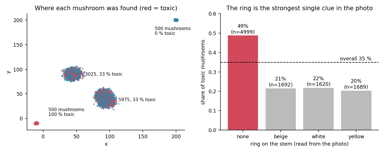
Map of the mushrooms and the effect of the ring

The mushrooms grow in four clumps. One clump of 500 mushrooms at $(-10,-10)$ is 100 % toxic, and another clump of 500 at $(200, 200)$ is 100 % edible. The two big clumps (9 000 mushrooms) both have exactly 33 % toxic mushrooms, and inside them, position tells you nothing. The test set has the same four clumps (250, 250, 1 489, 3 011 mushrooms). So 10 % of the test is free, and the real work is in the two big clumps.

The photos. They are not real photographs. They are flat-colour drawings, 500 × 300 pixels, with no anti-aliasing: in all of them together there are only 27 distinct colours.

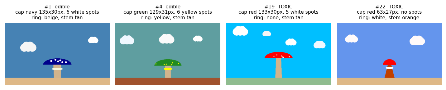
Four drawings and what our parser reads from them

Every drawing follows one template: a sky (6 possible colours), clouds, a ground strip (9 colours) starting at row 264, and a mushroom standing on column 250. The mushroom has a cap (navy, green or red, of variable width and height), white or yellow spots on the cap (0 to 13 of them), maybe a ring around the stem (beige, white or yellow), and a stem (tan, sienna or orange) that may widen towards the ground.

With such images you do not need a neural network. You can read the drawing exactly, the way the program that made it wrote it. Our parser walks down column 250. The first cap-coloured pixel marks the top of the cap. The cap ends where the stem colour starts. Any other colour crossing column 250 below the cap is the ring. Spots are the white or yellow pixels inside the cap's outline, counted as connected blobs. Widths are horizontal runs of one colour through column 250. Why insist on column 250, rather than just "everything that is not sky"? Because clouds often touch the mushroom, and a first version that took the whole non-sky blob reported white caps and phantom rings on about 10 % of the images. Reading along the axis of symmetry avoids the clouds completely.

The ring alone already moves the toxic rate from 49 % (no ring) to about 21 % (any ring), as the right panel above shows.

A first baseline

Using the table only, with categorical columns one-hot encoded:

model (table only)	CV AUC	score
logistic regression	0.698	39.5
gradient-boosted trees, default settings	0.760	52.0
gradient-boosted trees, tuned	0.775	55.0

Gradient boosting on the table alone already clears the 40-point threshold, and it beats logistic regression by 6 points of AUC. That gap is a first clue: something in this data is not additive. The image features alone give only 0.707. Put the two together and the AUC jumps to 0.933. That sum is far larger than either part, and that tells you where the key idea lies.

The key idea

Toxicity is decided by rules that combine table columns and drawing features, and those rules contain interactions where one feature reverses the effect of another. A model that adds up effects cannot see them. A model that splits on one feature after another can.

Look inside the two big clumps and split them by the ring:

Interactions behind toxicity

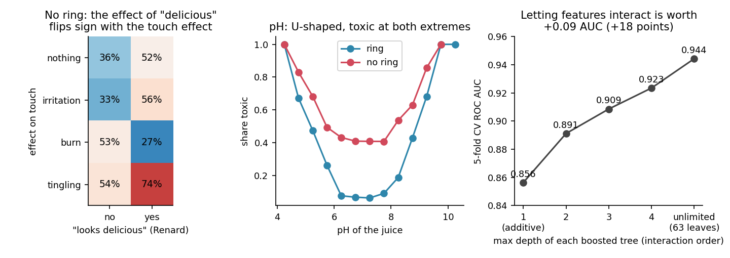
Left panel (mushrooms without a ring). If touching the mushroom does nothing or irritates, "looks delicious" makes it more likely toxic (36 % to 52 %, 33 % to 56 %). If it burns, "looks delicious" makes it less likely toxic (53 % to 27 %). This is an XOR-like pattern. Averaged over all touch effects, "looks delicious" barely matters (AUC 0.52 on its own), yet once you know the touch effect it moves the toxic rate by 20 to 25 points.
Middle panel (pH of the juice). The curve is a U: below pH 5 or above pH 9.5, almost every mushroom is toxic, whatever else you know. A linear term in pH can only say "higher is worse" or "lower is worse", so it misses half of the effect. The U is also much deeper for mushrooms with a ring (6 % toxic near neutral pH) than without (41 %): the ring and the pH interact too.
And so on. Within the ring group, the number of spots and the presence of insects matter. Within the no-ring group, the stem colour and the cap width matter. The important features are not the same in the two branches.

Why do trees catch this when a linear model cannot? A logistic regression models $\text{logit}\,p = \sum_j f_j(x_j)$ : each feature pushes the odds by an amount that does not depend on the other features. Even with flexible splines for each $f_j$ , which handle the U-shape, it cannot represent "delicious helps if it burns, hurts otherwise". That requires a term in two features at once, $f(x_{\text{touch}}, x_{\text{delicious}})$ . A decision tree builds such terms naturally: after splitting on the ring and then on the touch effect, a split on "delicious" in one branch can go the opposite way from the same split in another branch. A tree of depth $d$ can express interactions of up to $d$ features.

The right panel measures exactly this. It shows gradient boosting with the depth of each tree capped. Depth 1 (stumps) gives an additive model, which scores 0.856, the same as our additive spline logistic regression (0.857). Each extra level of allowed interaction adds AUC: depth 2 gives 0.891, depth 4 gives 0.923, and trees with 63 leaves give 0.944. Interactions are worth about 0.09 AUC here, or 18 points of the final score.

The full solution

Parse each drawing into 19 numbers (about 1 minute for all 15 000 images on 2 cores): cap colour, height and width; number, colour and total area of the spots; ring colour, height, width and position along the stem; stem colour, height and widths at the top, middle and bottom; sky colour, ground colour, number of clouds. The core of the parser is "walk down the axis of symmetry":

centre = C[:GROUND, CX]                          # colours along column 250, top to bottom
c0 = np.where(np.isin(centre, list(CAPS)))[0][0] # first cap pixel
...
below = centre[c1:]                              # from under the cap down to the ground
ring_rows = np.where(below != stem)[0]           # anything that is not stem colour = the ring

Join with the table. We also tried five hand-made features: $|\text{pH}_{\text{juice}} - 7.2|$ (the U turned into a slope), a ring flag, the pH difference between juice and soil, the cap's aspect ratio, and how much the stem flares. They brought nothing (0.944 with them, 0.945 without), because trees with enough leaves rebuild such features on their own. So the final model uses the raw columns plus the parsed drawing.
Gradient-boosted trees (HistGradientBoostingClassifier, native categorical handling): 400 rounds, learning rate 0.02, up to 63 leaves per tree, at least 20 mushrooms per leaf, L2 regularisation 1. We chose these with a small grid search scored by 5-fold CV. The clearest lesson of the grid: more leaves per tree always helped (7 leaves: 0.920, 15: 0.935, 31: 0.941, 63: 0.944), while the learning rate and the number of rounds barely mattered once there were enough of them. Bigger trees mean deeper interactions, which confirms the key idea.
Predict the test probabilities with the model refitted on all 10 000 mushrooms. The script writes y_test.csv in the submission format, but we did not submit it.

Several things turned out not to matter, which is useful to know: the sky colour, the ground colour, the clouds, the stem height, odour, texture, weight, porosity and soil temperature. Dropping all of them changed the CV AUC by at most 0.003, which is within the noise. They are most likely decoys from the data generator.

Results

Scores are 5-fold cross-validated ROC AUC on the 10 000 training mushrooms, plus the score on a held-out 20 % split (2 000 mushrooms) for the final model. The official test labels are private.

approach	AUC	score
logistic regression, table only	0.698	39.5
gradient boosting, table only, default	0.760	52.0
gradient boosting, table only, tuned	0.775	55.0
gradient boosting, drawing features only	0.707	41.4
gradient boosting, table + ring position only	0.861	72.3
logistic regression, table + drawing (linear)	0.802	60.4
logistic regression with splines, table + drawing (additive)	0.857	71.3
boosting with depth-1 trees (additive)	0.856	71.3
single decision tree, depth 10	0.900	80.0
boosting, depth 2 / depth 3 / depth 4	0.891 / 0.909 / 0.923	78.2 / 81.7 / 84.7
boosting, 15 leaves	0.933	86.6
random forest, 500 trees	0.936	87.2
boosting, 63 leaves + 5 hand-made features	0.944	88.9
boosting, 63 leaves (final), 5-fold CV	0.945	89.0
same model, held-out 20 % split	0.948	89.6

The final model reaches AUC 0.945 in cross-validation (score 89.0) and 0.948 on the held-out split (score 89.6), more than twice the 40-point qualification threshold. With 2 000 held-out mushrooms, the standard error of an AUC near 0.95 is about 0.005, so the two numbers agree.

What to remember

Look at the images before reaching for a CNN. Synthetic, flat-colour pictures can be read exactly with a few lines of NumPy, which is faster, more precise and more robust than any learned model. Check the number of distinct colours: here it was 27.
When the parts score less than the whole, look for interactions. Table alone 0.78, image alone 0.71, together 0.93. Single-feature AUCs near 0.5 do not mean a feature is useless: "looks delicious" scores 0.52 alone but flips the risk by 25 points once you know the touch effect.
Tree depth is interaction order. Boosting with stumps is an additive model. Raising the depth (or the number of leaves) lets the model combine more features, and watching the CV score rise with depth is a direct test for interactions.
Turn U-shapes into slopes for linear models. $|x - x_0|$ lets a linear model capture a risk that rises at both extremes, like the pH here. A tree does not need it: it simply splits twice.
Check the train/test match early. An adversarial-validation AUC of 0.49 told us a random validation split was trustworthy. The 1 000 mushrooms in the pure clumps were a free 10 %, worth spotting with one scatter plot.

"""OFIA 2025, stage 1: "Mushroom Mission on ExoMycelia-7", worked solution.

Idea: the photos are flat-colour synthetic drawings, so we do not need a CNN. We READ each drawing
(cap colour and size, spots, ring, stem) into a handful of numbers, join them to the table, and let
gradient-boosted trees find the strongly non-additive rules (XOR-like interactions) behind toxicity.

Usage:  python solution.py [path/to/OFIA_2025_epreuve_1]
Prints the 5-fold CV AUC and the AUC on a held-out 20 % split (official test labels are private),
then writes y_test.csv in the submission format (id, probabilite_toxique).
"""
import sys
from multiprocessing import Pool

import numpy as np
import pandas as pd
from PIL import Image
from scipy import ndimage
from sklearn.ensemble import HistGradientBoostingClassifier
from sklearn.metrics import roc_auc_score
from sklearn.model_selection import StratifiedKFold, cross_val_predict, train_test_split

ROOT = sys.argv[1] if len(sys.argv) > 1 else "work/OFIA_2025_epreuve_1"
CAPS = {0x00008B: "navy", 0x228B22: "green", 0xFF0000: "red"}
STEMS = {0xA0522D: "sienna", 0xC04000: "orange", 0xD2B48C: "tan"}
DECO = {0xFFFFFF: "white", 0xFFFF00: "yellow", 0xF5F5DC: "beige"}   # spot and ring colours
CLOUDS = [0xFFFFFF, 0xFFFAFA, 0xFAFAFA, 0xF0F8FF, 0xF5F5F5]
CX, GROUND = 250, 264   # every mushroom stands on column 250; the ground starts at row 264


# ------------------------------------------------------------------ 1. reading a drawing
def run_len(row, x, colour):
    """Length of the horizontal run of `colour` that passes through column x."""
    if row[x] != colour:
        return 0
    left, right = x, x
    while left > 0 and row[left - 1] == colour:
        left -= 1
    while right < len(row) - 1 and row[right + 1] == colour:
        right += 1
    return right - left + 1


def parse(path):
    rgb = np.array(Image.open(path).convert("RGB")).astype(np.int64)
    C = rgb[..., 0] * 65536 + rgb[..., 1] * 256 + rgb[..., 2]      # one integer per colour
    centre = C[:GROUND, CX]
    f = {}
    # cap: from the first cap-coloured pixel of the centre column down to the stem
    c0 = np.where(np.isin(centre, list(CAPS)))[0][0]
    cap = centre[c0]
    c1 = c0 + 1
    while c1 < GROUND and centre[c1] in (cap, *DECO):   # a spot may sit on the centre column
        c1 += 1
    stem = C[GROUND - 1, CX]
    f["cap_color"], f["stem_color"] = CAPS[cap], STEMS.get(stem, "other")
    f["cap_h"] = c1 - c0
    # spots = decoration colours strictly inside the cap outline, row by row
    spots = np.zeros(C.shape, bool)
    widths = []
    for r in range(c0, c1):
        xs = np.where(C[r] == cap)[0]
        if len(xs):
            spots[r, xs.min():xs.max() + 1] = np.isin(C[r, xs.min():xs.max() + 1], list(DECO))
            widths.append(xs.max() - xs.min() + 1)
    f["cap_w"] = max(widths)
    f["n_spots"] = ndimage.label(spots)[1]
    f["spot_area"] = int(spots.sum())
    if f["n_spots"]:
        u, k = np.unique(C[spots], return_counts=True)
        f["spot_color"] = DECO[u[k.argmax()]]
    else:
        f["spot_color"] = "none"
    # ring = a non-stem colour crossing the centre column between the cap and the ground
    below = centre[c1:]
    ring_rows = np.where(below != stem)[0]
    if len(ring_rows):
        rc = below[ring_rows[0]]
        f["ring_color"] = DECO.get(rc, "other")
        f["ring_h"] = len(ring_rows)
        f["ring_w"] = max(run_len(C[c1 + r], CX, rc) for r in ring_rows)
        f["ring_pos"] = ring_rows.mean() / len(below)       # 0 = right under the cap
    else:
        f["ring_color"], f["ring_h"], f["ring_w"], f["ring_pos"] = "none", 0, 0, -1.0
    f["stem_h"] = GROUND - c1
    f["stem_w_top"] = run_len(C[c1 + 1], CX, stem)
    f["stem_w_mid"] = run_len(C[(c1 + GROUND) // 2], CX, stem)
    f["stem_w_bot"] = run_len(C[GROUND - 1], CX, stem)
    # background (turns out to carry no signal, kept for completeness)
    vals, cnt = np.unique(C[:GROUND], return_counts=True)
    f["sky"], f["ground"] = "%06x" % vals[cnt.argmax()], "%06x" % C[-1, 0]
    white = np.isin(C[:GROUND], CLOUDS) & ~spots[:GROUND]
    lab, n = ndimage.label(white)
    sizes = ndimage.sum(white, lab, range(1, n + 1)) if n else []
    f["n_clouds"] = int(sum(s > 300 for s in sizes))
    return f


def load(split):
    tab = pd.read_csv(f"{ROOT}/X_{split}.csv")
    with Pool(2) as pool:
        img = pd.DataFrame(pool.map(parse, [f"{ROOT}/images/{split}/champignon_{i}.png" for i in tab.id],
                                    chunksize=50))
    D = pd.concat([tab.drop(columns="id"), img], axis=1)
    # Engineered features such as |pH - 7.2| or a ring flag were tried: no gain, the trees find them.
    for c in D:
        if not pd.api.types.is_numeric_dtype(D[c]):
            D[c] = D[c].astype("category")
    return tab.id.values, D


# ------------------------------------------------------------------ 2. model
def model():
    return HistGradientBoostingClassifier(
        categorical_features="from_dtype", max_iter=400, learning_rate=0.02, max_leaf_nodes=63,
        min_samples_leaf=20, l2_regularization=1.0, early_stopping=False, random_state=0)


if __name__ == "__main__":
    _, D = load("train")
    y = pd.read_csv(f"{ROOT}/y_train.csv").est_toxique.values
    test_ids, T = load("test")
    T = T.astype({c: pd.CategoricalDtype(D[c].cat.categories) for c in D if str(D[c].dtype) == "category"})

    final = lambda auc: (auc - 0.5) * 200                        # official score formula
    p = cross_val_predict(model(), D, y, cv=StratifiedKFold(5, shuffle=True, random_state=0),
                          method="predict_proba")[:, 1]
    auc = roc_auc_score(y, p)
    print(f"5-fold CV      AUC {auc:.4f}  score {final(auc):.1f}")

    a, b, ya, yb = train_test_split(D, y, test_size=0.2, stratify=y, random_state=42)
    auc = roc_auc_score(yb, model().fit(a, ya).predict_proba(b)[:, 1])
    print(f"held-out 20 %  AUC {auc:.4f}  score {final(auc):.1f}")

    m = model().fit(D, y)
    pd.DataFrame({"id": test_ids, "probabilite_toxique": m.predict_proba(T)[:, 1]}).to_csv(
        "y_test.csv", index=False)
    print("wrote y_test.csv")