IOAI Training: Learn AI by solving problems

The problem in brief

Every test file is one second of audio (16 000 samples at 16 kHz) that is the exact sum of two real environmental recordings: waves with a campfire, birds with footsteps, rain with a dog. You must give back both original waveforms. For training you get 3 000 mixtures together with their two sources; the 400 test mixtures use recordings that never appear in training. This is blind source separation, and since the two outputs are unordered, the metric tries both pairings.

The test sources are hidden on Kaggle and we never submitted anything. All scores below come from our own validation: we hold out 30 % of the distinct source recordings and evaluate on the 258 training mixtures made only of those held-out recordings, so that, as on the test set, the validation sounds were never heard during training.

How you are scored

For each clip with true sources $s_1, s_2$ and outputs $p_1, p_2$ ,

\text{err} = \min\big(\text{MSE}(s_1,p_1) + \text{MSE}(s_2,p_2),\ \text{MSE}(s_1,p_2) + \text{MSE}(s_2,p_1)\big),

with MSE averaged over the 16 000 samples, and the score is the mean of err over the clips: the permutation-invariant MSE (PIT-MSE), lower is better. The statement gives two landmarks: outputting silence scores about 0.020, and outputting half of the mixture for both sources about 0.010. Real separation means going below 0.010.

What to aim for. On the public leaderboard, the organisers' reference solution scores 0.00516, the best contestant 0.00629, and several teams sit at the half-mixture level 0.01002.

First look at the data

Every source has exactly the same loudness: its root-mean-square amplitude is 0.1 in all 6 000 training sources (the statement calls them "loudness-normalised"). That explains the landmarks: silence costs $0.1^2 + 0.1^2 = 0.02$ , and half of the mixture costs half of that when the two sources are uncorrelated.
Sources are reused. The 6 000 source slots of the training set contain only 1 558 distinct recordings: the organisers built the 3 000 mixtures by pairing the same clips in different ways. Two consequences. A random validation split of the mixtures would leak (the same sound in training and validation), so we split by recording. And the training set is really "1 558 sounds that you may combine as you like".
The sounds are varied textures: broadband noise (rain, waves, wind), harmonic sounds (birds, engines), impulsive events (footsteps, knocks). Their spectrograms overlap but rarely occupy the same time-frequency cells with the same strength.

A first baseline

The organisers' baseline outputs half of the mixture twice: PIT-MSE 0.0100, which, by construction, separates nothing. Every competitor who kept it sits at 0.01002 on the leaderboard.

The key idea

Two ideas together: separate by masking the spectrogram, learned end to end on the metric itself, and train on freshly invented mixtures, by summing random pairs of training sources, instead of only the 3 000 given ones.

Masking. In a short-time Fourier transform (STFT) the two sounds usually dominate different time-frequency cells. A network looks at the log-magnitude spectrogram of the mixture and outputs, for every cell $(f,t)$ , two weights $m_1, m_2 \ge 0$ with $m_1 + m_2 = 1$ (a softmax). Each estimate is the mixture's complex STFT multiplied by its mask and turned back into a waveform:

\hat s_k = \text{iSTFT}\big(m_k \odot X\big), \qquad X = \text{STFT}(x),\qquad k = 1, 2 .

Because the masks sum to one, the two estimates always add up exactly to the mixture, a constraint the true sources also satisfy. The whole chain, STFT, network, mask, inverse STFT, is differentiable, so we train directly with the PIT-MSE on the waveforms: the loss is the competition metric, and taking the minimum over the two pairings lets the network output the sources in any order (permutation-invariant training).

Dynamic mixing. A mixture is just the sum of two sources, so we can make as many new training examples as we want: at every step, draw two random recordings from the training pool, shift one of them circularly by a random amount, and add them. With 1 060 training recordings that is over half a million possible pairs, times 16 000 shifts, instead of 1 543 fixed mixtures. The network can no longer memorise the training mixtures; it has to learn what a single source looks like. The left panel below shows the difference with the same network and the same 12-minute budget: on the fixed mixtures, the validation error plateaus around 0.0069 to 0.0070 and then creeps back up (0.0072 at the end) as the network memorises its 1 543 examples, while with dynamic mixing it keeps falling (0.0061).

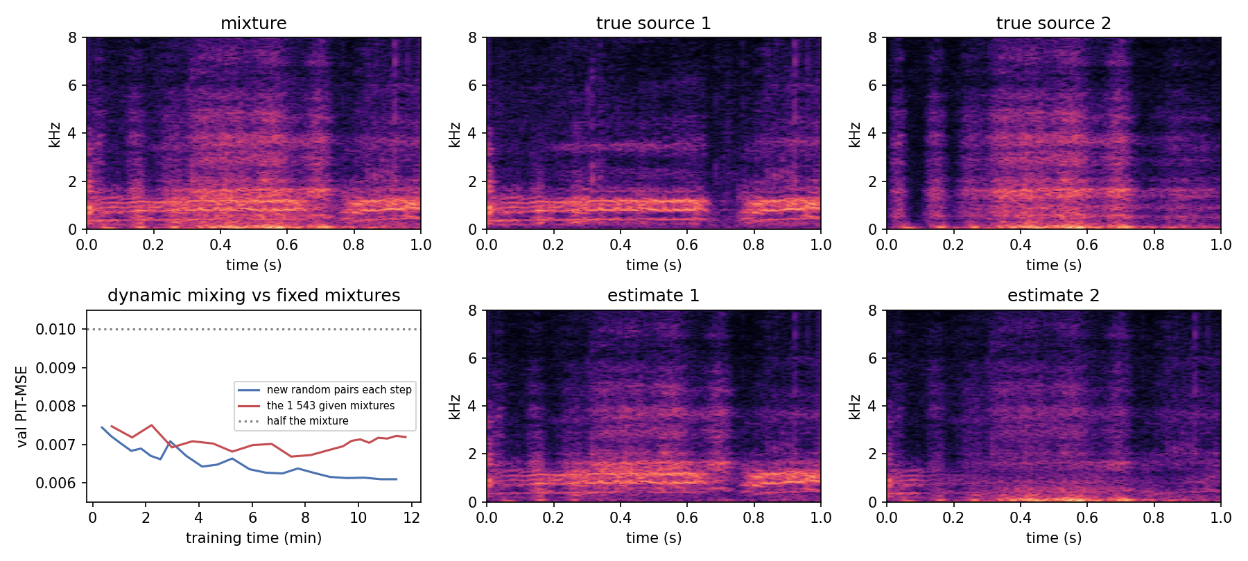
Separation of a validation mixture and learning curves

On the right, a held-out mixture of a hum with strong harmonics below 1.5 kHz (source 1) and a broadband noisy sound (source 2): the first estimate keeps the harmonic lines and the gap at 0.7 s, the second keeps the broadband part. The separation is not perfect (some of each sound leaks into the other), but this example's error is 0.0048, half of the half-mixture baseline.

The full solution

STFT with a 512-sample Hann window (32 ms) and a hop of 128 samples, giving 257 frequencies × 126 frames; input feature $\log(1 + 10\,|X|)$ .
A small 2D U-Net: four levels (16, 32, 64, 128 channels, two 3 × 3 convolutions with batch normalisation each), max-pooling on the way down, bilinear upsampling and skip connections on the way up, a final 1 × 1 convolution to 2 channels and a softmax over them.
Training: batches of 8 freshly mixed pairs, AdamW (learning rate $10^{-3}$ with a cosine decay over the time budget), PIT-MSE on the waveforms; 12 minutes for validation, 15 minutes on all 1 558 recordings for the final model.
Inference: the two masked, inverted signals, written as Base85 float32 strings.

X = stft(mix)
m = net(torch.log1p(X.abs() * 10)[:, None])                 # (B, 2, F, T), m[:,0] + m[:,1] = 1
est = torch.stack([istft(X * m[:, k]) for k in range(2)], 1)
loss = pit_mse(est, sources).mean()                          # the metric itself

Results

approach (validation: 258 mixtures of unseen recordings)	PIT-MSE
silence	0.0200
half of the mixture twice (organisers' baseline)	0.0100
U-Net masks, trained on the 1 543 fixed training mixtures	0.0072 (best 0.0069 mid-training)
U-Net masks, dynamic mixing (final recipe)	0.0061
same, outputs rescaled towards the known loudness 0.1	0.0060 to 0.0065

Our model reaches a PIT-MSE of 0.0061 on validation mixtures of unseen recordings, better than the best contestant on the public leaderboard (0.00629) and behind the organisers' reference (0.00516). The comparison is indicative, since the leaderboard uses other clips.

One more experiment teaches something about MSE. Since every true source has RMS 0.1, we tried rescaling each estimate to that loudness. It does not help: our estimates have a median RMS of 0.084, and pushing them to 0.1 makes the error worse (0.0065); only a gentle partial rescaling gains a negligible 0.00005. Under squared error, when you are unsure, it pays to shrink your estimate towards zero: the network has learned to be quieter than the truth on purpose, exactly like a regression that predicts the mean.

What to remember

Masks in the time-frequency domain are the classic tool for audio separation: sounds that overlap in time rarely overlap in every frequency, and a softmax mask keeps the estimates consistent with the mixture.
Train on the metric. STFT and inverse STFT are differentiable, so you can optimise the waveform PIT-MSE directly; the min over pairings removes the arbitrary order of the outputs.
When the data is a sum, invent more sums. Dynamic mixing turned 1 543 mixtures into an endless stream and was the biggest single gain against overfitting.
Split validation by the real unit of independence. Here the same recordings were reused across mixtures, so the split had to be by recording, as for patients or speakers elsewhere.
MSE likes shrinkage. Matching the known loudness looks principled but hurts; uncertain estimates should be conservative.

"""Audio Demixing (Tenerife camp 2026, day 7): split 1 s of 16 kHz audio into the two environmental
recordings that were summed to make it. Metric: permutation-invariant MSE (lower is better).

Data: audio-demix-data/ from the Kaggle competition spain-camp-day7-audio. Run once with any mode to
cache the wavs as .npy. Test sources are hidden: `python solution.py 12 val` holds out 30 % of the
unique source recordings (and every mixture that uses only them) and reports the PIT-MSE there;
`python solution.py 15 full` trains on everything and writes submission.csv. First argument = minutes.

Method: a small U-Net predicts two soft masks (softmax, so they sum to one) on the log-magnitude STFT;
masks x complex mixture STFT -> inverse STFT -> two waveforms; trained end to end with the PIT-MSE
itself, on *dynamically remixed* pairs of training sources (a new random pair and shift at every step).
"""
import os, sys, time, math, base64
os.environ["OMP_NUM_THREADS"] = "2"
import numpy as np, pandas as pd, soundfile as sf, torch, torch.nn as nn, torch.nn.functional as F
torch.set_num_threads(2); torch.manual_seed(0); np.random.seed(0)
dev = "mps" if torch.backends.mps.is_available() else "cpu"
if dev == "mps": torch.mps.set_per_process_memory_fraction(0.1)
MINUTES = float(sys.argv[1]); MODE = sys.argv[2]          # "val" or "full"
DYN = sys.argv[3] == "dyn" if len(sys.argv) > 3 else True
D = "audio-demix-data"
if not os.path.exists("M.npy"):
    tr, te = pd.read_csv(f"{D}/train.csv"), pd.read_csv(f"{D}/test.csv")
    rd = lambda f: sf.read(f"{D}/{f}", dtype="float32")[0]
    for name, files in [("M", tr.file), ("S1", tr.sig_1), ("S2", tr.sig_2), ("T", te.file)]:
        np.save(f"{name}.npy", np.stack([rd(f) for f in files]))
M = np.load("M.npy"); S1 = np.load("S1.npy"); S2 = np.load("S2.npy")

# ---- identify unique source recordings, split them so validation sources are never seen ----
key = lambda x: x[:400].tobytes()
uid = {}
src_id = np.array([[uid.setdefault(key(a), len(uid)) for a in (s1, s2)] for s1, s2 in zip(S1, S2)])
n_src = len(uid)
rng = np.random.default_rng(0)
val_src = rng.random(n_src) < 0.3 if MODE == "val" else np.zeros(n_src, bool)
is_val = val_src[src_id].all(1); is_tr = (~val_src[src_id]).all(1)
pool = {}
for i in np.where(is_tr)[0]:
    for k, s in zip(src_id[i], (S1[i], S2[i])): pool[k] = s
POOL = torch.tensor(np.stack(list(pool.values())))
print(f"unique sources {n_src}, train pool {len(POOL)}, val mixtures {is_val.sum()}, train mixtures {is_tr.sum()}", flush=True)

NFFT, HOP = 512, 128
WIN = torch.hann_window(NFFT).to(dev)
stft = lambda x: torch.stft(x, NFFT, HOP, window=WIN, return_complex=True)
istft = lambda X: torch.istft(X, NFFT, HOP, window=WIN, length=16000)

def cbr(i, o): return nn.Sequential(nn.Conv2d(i, o, 3, padding=1), nn.BatchNorm2d(o), nn.ReLU(), nn.Conv2d(o, o, 3, padding=1), nn.BatchNorm2d(o), nn.ReLU())
class UNet(nn.Module):
    """log-magnitude spectrogram -> 2 soft masks that sum to one"""
    def __init__(s, c=16):
        super().__init__()
        s.d1, s.d2, s.d3, s.d4 = cbr(1, c), cbr(c, 2 * c), cbr(2 * c, 4 * c), cbr(4 * c, 8 * c)
        s.u3, s.u2, s.u1 = cbr(12 * c, 4 * c), cbr(6 * c, 2 * c), cbr(3 * c, c)
        s.out = nn.Conv2d(c, 2, 1)
    def forward(s, x):
        H, W = x.shape[-2:]
        x = F.pad(x, (0, (-W) % 8, 0, (-H) % 8))
        a = s.d1(x); b = s.d2(F.max_pool2d(a, 2)); c = s.d3(F.max_pool2d(b, 2)); d = s.d4(F.max_pool2d(c, 2))
        up = lambda t, r: F.interpolate(t, size=r.shape[-2:], mode="bilinear", align_corners=False)
        c = s.u3(torch.cat([up(d, c), c], 1)); b = s.u2(torch.cat([up(c, b), b], 1)); a = s.u1(torch.cat([up(b, a), a], 1))
        return torch.softmax(s.out(a), 1)[..., :H, :W]

def separate(net, mix):
    X = stft(mix)
    m = net(torch.log1p(X.abs() * 10)[:, None])
    return torch.stack([istft(X * m[:, k]) for k in range(2)], 1)

def pit_mse(est, s):
    e1 = ((est[:, 0] - s[:, 0]) ** 2).mean(1) + ((est[:, 1] - s[:, 1]) ** 2).mean(1)
    e2 = ((est[:, 0] - s[:, 1]) ** 2).mean(1) + ((est[:, 1] - s[:, 0]) ** 2).mean(1)
    return torch.minimum(e1, e2)

net = UNet().to(dev)
opt = torch.optim.AdamW(net.parameters(), lr=1e-3, weight_decay=1e-4)
BS = 8; t0 = time.time(); step = 0
tr_idx = np.where(is_tr)[0]
def batch():
    if DYN:   # dynamic mixing: two random training sources, random circular shift
        i, j = torch.randint(len(POOL), (BS,)), torch.randint(len(POOL), (BS,))
        a, b = POOL[i], POOL[j]
        b = torch.roll(b, int(np.random.randint(16000)), 1)
        return torch.stack([a, b], 1)
    k = np.random.choice(tr_idx, BS)
    return torch.tensor(np.stack([S1[k], S2[k]], 1))
def evaluate():
    net.eval(); E = []
    with torch.no_grad():
        for i in range(0, is_val.sum(), 32):
            k = np.where(is_val)[0][i:i + 32]
            est = separate(net, torch.tensor(M[k]).to(dev))
            E.append(pit_mse(est, torch.tensor(np.stack([S1[k], S2[k]], 1)).to(dev)).cpu().numpy())
    net.train(); return float(np.concatenate(E).mean())
total = MINUTES * 60
while time.time() - t0 < total:
    frac = (time.time() - t0) / total
    for g in opt.param_groups: g["lr"] = 1e-3 * 0.5 * (1 + math.cos(math.pi * frac))      # cosine decay over the time budget
    s = batch().to(dev); mix = s.sum(1)
    loss = pit_mse(separate(net, mix), s).mean()
    opt.zero_grad(); loss.backward(); opt.step(); step += 1
    if step % 500 == 0:
        msg = f"step {step} {time.time()-t0:.0f}s loss {loss.item():.5f}"
        if MODE == "val": msg += f" val PIT-MSE {evaluate():.5f}"
        print(msg, flush=True)
from safetensors.torch import save_file; save_file({k: v.contiguous().cpu() for k, v in net.state_dict().items()}, f"unet_{MODE}_{'dyn' if DYN else 'fixed'}.safetensors")
if MODE == "full":   # write the submission
    T = np.load("T.npy"); net.eval(); out = []
    with torch.no_grad():
        for i in range(0, len(T), 32):
            out.append(separate(net, torch.tensor(T[i:i + 32]).to(dev)).cpu().numpy())
    out = np.concatenate(out).astype("<f4")
    enc = lambda x: base64.b85encode(x.tobytes()).decode("ascii")
    ids = pd.read_csv(f"{D}/test.csv").ID
    pd.DataFrame({"ID": ids, "sig_1": [enc(o[0]) for o in out], "sig_2": [enc(o[1]) for o in out]}).to_csv("submission.csv", index=False)
    print("wrote submission.csv", out.shape)
if MODE == "val": print("final val PIT-MSE", evaluate(), "| half-mix on val", float(((np.stack([S1, S2], 1)[is_val] - M[is_val, None] / 2) ** 2).mean(2).sum(1).mean()))