IOAI Training: Learn AI by solving problems

The problem in brief

A camp kitchen receives crates of hazelnuts and wants the bad ones caught before lunch. You get 431 photographs of healthy nuts only, no example of a defect and no label of any kind, and 70 photographs of nuts that all have at least one defect of an undisclosed type. For each test photo (1024 × 1024 pixels) you must produce an anomaly map: a 1024 × 1024 image of values from 0 ("certainly normal") to 255 ("certainly a defect"), so the task is unsupervised defect localisation, pixel by pixel. One rule makes it a real contest: the only pretrained network allowed is a ResNet-18 trained on ImageNet-1k.

How we evaluate. The hidden masks are not on Kaggle, and we never submitted anything. But the statement says the images are the hazelnut category of the public MVTec Anomaly Detection dataset, whose ground-truth masks are published. We downloaded that category from a public Hugging Face mirror (foersben/mvtec-ad) and matched every one of the 70 test images to an MVTec test image: all 70 are pixel-for-pixel identical to a distinct MVTec image (18 cracks, 17 cuts, 18 holes, 17 prints), so we rebuilt the official ground truth exactly and scored with our own implementation of the competition metric (it gives exactly 0.15 for a constant map, as the statement says it should). These masks were used only for scoring. The one setting we compared on them, the input resolution, was chosen on the odd-numbered images and checked on the even-numbered ones.

How you are scored

The metric is AUPRO, the area under the per-region-overlap curve. Each connected component of the true defect masks is a region $R_k$ (136 regions in the 70 images). At every threshold $t$ (0 to 255), the flagged pixels $P(t)$ are those with score $\ge t$ , and

\text{PRO}(t) = \frac{1}{K}\sum_{k=1}^{K} \frac{|P(t)\cap R_k|}{|R_k|}, \qquad \text{FPR}(t) = \frac{|P(t)\cap N|}{|N|},

where $N$ is the set of all normal pixels of all test images. The PRO-versus-FPR curve is integrated up to FPR 0.3 and normalised:

\text{AUPRO} = \frac{1}{0.3}\int_0^{0.3} \text{PRO}\; d(\text{FPR}).

Three consequences drive the whole solution. Every defect region counts the same, so a tiny scratch matters as much as a huge crack. Only the low false-positive part of the curve counts. And thresholds are shared by all images, so the scores must be on one common scale: normalising each map separately would destroy the ranking between images.

What to aim for. A constant map scores 0.15. The organisers' colour baseline scores 0.672 on the public half of the test set, and the best public leaderboard score is 0.972 (on 35 of the 70 images).

First look at the data

The pictures are taken in a fixed setup: one nut on a black background, centred, under constant lighting, but in any orientation, which is what makes "normal" rich: the striped shell and the rough base can appear anywhere. The defects are small or large: a fine cut covers 0.2 % of the image, a broken shell almost 28 %. Some defects, like the "print" class (a white mark drawn on the shell), change colour; others, like cuts and cracks, change texture and shape but barely the colour.

A first baseline

The organisers' starter notebook fits a Gaussian to the RGB colour of training pixels and scores every pixel by its Mahalanobis distance to that colour model,

d(x) = \sqrt{(x-\mu)^\top \Sigma^{-1} (x-\mu)} .

On the 70 images it scores AUPRO 0.746. It finds white prints and dark holes, but a pixel's colour says nothing about texture or shape: a cut has the same brown as the rest of the shell, and the bright base of a healthy nut looks just as "abnormal" as a defect.

The key idea

Describe every small patch of an image by pretrained CNN features, keep a memory of all the patches seen on healthy nuts, and call a test patch anomalous if even its nearest healthy neighbour is far away. This is PatchCore (Roth et al., 2022), and it needs no training at all.

Why pretrained features? The mid-level layers of an ImageNet CNN respond to edges, textures and small shapes: exactly the vocabulary needed to tell a smooth striped shell from a crack. We use layer2 (128 channels, one vector every 8 pixels) and layer3 (256 channels, every 16 pixels, upsampled to the same grid), each averaged over its 3 × 3 neighbours so that a vector describes a small neighbourhood, giving a 384-dimensional descriptor per patch. Deeper layers are too tied to ImageNet classes, shallower ones too local.
Why nearest neighbour? A healthy patch of a test nut looks like some patch of some training nut, maybe at another place and in another orientation. So rather than modelling "normal" with one Gaussian, we keep all the healthy patches and use the distance to the closest one,

s(\text{patch}) = \min_{m \in \mathcal M} \lVert \phi(\text{patch}) - m \rVert_2 ,

which handles a very multi-modal normal class (shell, stripes, base, tip, background) for free.

Why a coreset? At 896 × 896 input, the 431 training nuts produce 5.4 million patches. We keep a random 25 %, then select 1.5 % of them (about 20 000) by greedy k-centre: repeatedly add the patch that is farthest from everything already chosen. Unlike random sampling, this keeps rare-but-normal appearances (an unusual angle of the base), which would otherwise become false positives.
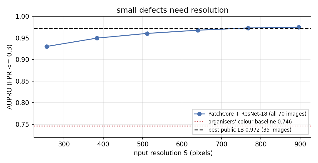
Why high resolution? A patch is $8$ pixels of the resized image. At 256 × 256 a patch covers 32 × 32 pixels of the original, so a 0.2 % cut fills only a small part of a patch and its signal is diluted. Raising the input size to 896 makes each patch cover about 9 × 9 original pixels, and AUPRO climbs steadily:

AUPRO against input resolution

Here is what the nearest-patch distance looks like on four test nuts (green and cyan: true defect outline):

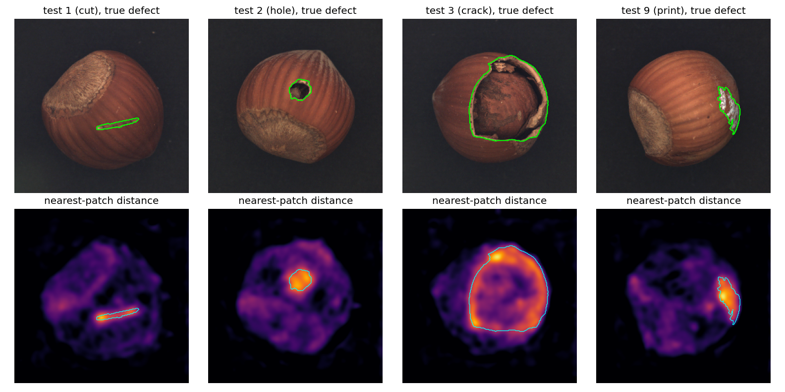
Test nuts, true defects and anomaly maps

The cut, the hole, the broken shell and the white print all light up, while the healthy shell stays dark; the brightest false alarms sit on the rough base and the edge of the shell, which vary most from nut to nut.

The full solution

Resize each image to 896 × 896, extract ResNet-18 layer2 and layer3, 3 × 3 average pooling, upsample layer3 to the layer2 grid (112 × 112), concatenate: 384 numbers per patch.
Memory bank: random 25 % of all training patches, then a greedy k-centre coreset of 1.5 % of them (computed on a random 128-dimensional projection, which preserves distances well enough for the selection and is much faster).
For each test patch, the Euclidean distance to its nearest neighbour in the bank; upsample the 112 × 112 map to 1024 × 1024 (bilinear) and smooth it with a Gaussian of $\sigma = 12$ pixels.
Convert to uint8 with one monotone mapping for the whole test split: the 256 levels are placed at the quantiles of all test scores from the 40th to the 100th percentile. AUPRO only depends on the order of the scores, and spreading the levels over the upper part of the distribution keeps the 256 thresholds where the curve is decided (FPR below 0.3).
Encode each map in Base85, 16 slices per image, as the statement requires.

d = torch.cdist(e.reshape(-1, 384), M).min(1).values.reshape(h, h)   # nearest healthy patch
up = F.interpolate(d[None, None], size=(1024, 1024), mode="bilinear")[0, 0]
amap = gaussian_filter(up.cpu().numpy(), 12)

The whole pipeline runs in under 2 minutes on the Apple GPU: about 20 s to embed the training nuts, a minute for the coreset, 30 s for the 70 test maps.

Results

approach (all 70 test images, rebuilt MVTec masks)	AUPRO
constant map (chance level)	0.150
RGB colour Mahalanobis distance (organisers' baseline)	0.746
PatchCore, 256 px, 2 % coreset, $\sigma = 16$	0.930
same, $\sigma = 8$ / $\sigma = 32$	0.931 / 0.926
same, 10 % coreset instead of 2 %	0.929
PatchCore at 384 / 512 / 640 / 768 px	0.950 / 0.960 / 0.968 / 0.973
PatchCore at 896 px, 1.5 % coreset of 25 % of the patches (final)	0.975
final, even-numbered images only (not used for the choice)	0.973

Our final maps reach AUPRO 0.975 on the 70 test images (0.973 on the half not used to pick the resolution), at the level of the best public leaderboard score (0.972, on half of the images). Two things did not matter: the blur width and the coreset size (2 % or 10 % give the same score: a small, well-spread memory is enough). One thing mattered a lot: resolution, worth +0.045. Going beyond 896 px (the original 1024) did not fit in our 2 GB GPU memory budget.

What to remember

Unsupervised anomaly detection = model the normal, flag the unusual. With only good examples, the question is never "what does a defect look like" but "how far is this from everything normal I have seen".
Pretrained mid-level CNN features plus nearest-neighbour distance are a remarkably strong, training-free detector, because a k-NN memory can represent a normal class with many modes.
Read the metric's fine print. AUPRO weights every region equally (so small defects matter, hence resolution) and sweeps global thresholds (so keep one score scale across images, never normalise each map on its own).
Use the order, not the values. A metric based on thresholds is invariant to monotone transforms; quantile-based quantisation spends the 256 levels where they count.
Check whether the data is public. Recognising MVTec AD let us rebuild the hidden ground truth and score honestly instead of guessing.

"""The Defected Nuts (Tenerife camp 2026, day 5): unsupervised pixel-level anomaly detection on
MVTec AD hazelnuts, scored by AUPRO (FPR <= 0.3). Only ResNet-18 (ImageNet-1k) may be used.

Data: defected-nuts-data/{train,test}/*.png from the Kaggle competition spain-camp-day5-cv;
ResNet-18 weights as safetensors (timm/resnet18.tv_in1k) in w/resnet18.safetensors.
The hidden masks are the public MVTec AD hazelnut ground truth: if gt_masks.npy (rebuilt by
matching every test image pixel for pixel to MVTec AD, see correction) is present, the script
also prints the AUPRO. It always writes submission.csv in the required Base85 format.

Method: PatchCore with a ResNet-18.
  1. every training image (resized to S x S) -> layer2 + layer3 feature maps, 3x3 average-pooled,
     layer3 upsampled to layer2's grid -> one 384-d vector per patch (stride 8 px of the resized image);
  2. memory bank = a random 25 % of all training patches, reduced to 1.5 % by greedy k-centre coreset;
  3. a test patch's anomaly score = distance to its nearest neighbour in the bank;
  4. upsample to 1024 x 1024, Gaussian blur, and one GLOBAL monotone map to uint8.
"""
import os, base64
os.environ.setdefault("OMP_NUM_THREADS", "2")
import numpy as np, pandas as pd, torch, timm, torch.nn.functional as F
from safetensors.torch import load_file
from PIL import Image
from scipy import ndimage
from scipy.ndimage import gaussian_filter

torch.set_num_threads(2); torch.manual_seed(0)
DEV = "mps" if torch.backends.mps.is_available() else "cpu"
if DEV == "mps": torch.mps.set_per_process_memory_fraction(0.1)
S, SUB, RATIO, SIGMA = 896, 0.25, 0.015, 12
D = "defected-nuts-data"

net = timm.create_model("resnet18", pretrained=False, features_only=True, out_indices=(2, 3))
net.load_state_dict({k: v for k, v in load_file("w/resnet18.safetensors").items() if not k.startswith("fc.")}, strict=False)
net = net.eval().to(DEV)
MEAN = torch.tensor([0.485, 0.456, 0.406], device=DEV).view(1, 3, 1, 1)
STD = torch.tensor([0.229, 0.224, 0.225], device=DEV).view(1, 3, 1, 1)


def load(p):
    a = np.asarray(Image.open(p).convert("RGB").resize((S, S), Image.BILINEAR))
    return torch.from_numpy(a.copy()).permute(2, 0, 1).float().div(255)


def embed(x):
    """(B, 3, S, S) -> (B, S/8, S/8, 384): mid-level features, each aware of its 3x3 neighbourhood"""
    with torch.no_grad():
        f2, f3 = net((x.to(DEV) - MEAN) / STD)
        f2, f3 = F.avg_pool2d(f2, 3, 1, 1), F.avg_pool2d(f3, 3, 1, 1)
        f3 = F.interpolate(f3, size=f2.shape[-2:], mode="bilinear", align_corners=False)
        return torch.cat([f2, f3], 1).permute(0, 2, 3, 1)


def memory_bank():
    bank = []
    for i in range(1, 432, 4):
        e = embed(torch.stack([load(f"{D}/train/{j}.png") for j in range(i, min(i + 4, 432))]))
        e = e.reshape(-1, e.shape[-1]).half().cpu()
        bank.append(e[torch.randperm(len(e))[:int(SUB * len(e))]])
    bank = torch.cat(bank)
    # greedy k-centre coreset: repeatedly add the patch farthest from everything chosen so far,
    # so rare-but-normal appearances are kept; done on a random 128-d projection for speed
    if DEV == "mps": torch.mps.empty_cache()
    P = torch.randn(bank.shape[1], 128) / 128 ** 0.5
    Zc = torch.cat([bank[i:i + 100000].float() @ P for i in range(0, len(bank), 100000)])
    zz = (Zc ** 2).sum(1).to(DEV); Z = Zc.half().to(DEV); del Zc
    d2 = lambda j: zz - 2 * (Z @ Z[j]).float() + zz[j]
    sel = [int(torch.randint(len(Z), (1,)))]; mind = d2(sel[0])
    for _ in range(int(RATIO * len(bank)) - 1):
        j = int(torch.argmax(mind)); sel.append(j); mind = torch.minimum(mind, d2(j))
    return bank[sel].float().to(DEV)


def score_map(p, M):
    e = embed(load(p)[None])[0]
    h = e.shape[0]
    d = torch.cdist(e.reshape(-1, M.shape[1]), M).min(1).values.reshape(h, h)
    up = F.interpolate(d[None, None], size=(1024, 1024), mode="bilinear", align_corners=False)[0, 0].cpu().numpy()
    return gaussian_filter(up, SIGMA)


def to_uint8(raw):
    """one monotone map for the whole test split (never per image): uniform levels over the top 60 %"""
    q = np.quantile(raw[:, ::8, ::8], np.linspace(0.4, 1, 256))
    return np.clip(np.searchsorted(q, raw) - 1, 0, 255).astype(np.uint8)


def aupro(maps, masks, fpr_max=0.3):
    """the competition metric: mean per-region overlap vs pooled FPR, integrated up to FPR 0.3"""
    hist_n, regions = np.zeros(256), []
    for m, g in zip(maps, masks):
        hist_n += np.bincount(m[~g].ravel(), minlength=256)
        lab, k = ndimage.label(g, structure=np.ones((3, 3)))
        regions += [np.bincount(m[lab == r], minlength=256) for r in range(1, k + 1)]
    fpr = np.cumsum(hist_n[::-1])[::-1] / hist_n.sum()
    pro = np.mean([np.cumsum(h[::-1])[::-1] / h.sum() for h in regions], 0)
    f, p = np.r_[0.0, fpr[::-1]], np.r_[0.0, pro[::-1]]
    j = int((f <= fpr_max).sum())
    fi, pi = f[:j], p[:j]
    if j < len(f):
        pi = np.r_[pi, p[j - 1] + (p[j] - p[j - 1]) * (fpr_max - f[j - 1]) / (f[j] - f[j - 1] + 1e-12)]
        fi = np.r_[fi, fpr_max]
    return np.trapezoid(pi, fi) / fpr_max


def mask_to_rows(image_id, mask, chunks=16, chunk_len=81920):
    s = base64.b85encode(mask.tobytes(order="C")).decode("ascii")
    return [((image_id - 1) * chunks + k + 1, chr(ord("A") + k) + s[k * chunk_len:(k + 1) * chunk_len]) for k in range(chunks)]


if __name__ == "__main__":
    M = memory_bank()
    maps = to_uint8(np.stack([score_map(f"{D}/test/{i}.png", M) for i in range(1, 71)]).astype(np.float32))
    if os.path.exists("gt_masks.npy"):
        gt = np.load("gt_masks.npy"); half = np.arange(70) % 2 == 1
        print("AUPRO all", round(aupro(list(maps), list(gt)), 4),
              "| even ids", round(aupro(list(maps[half]), list(gt[half])), 4))
    rows = [{"id": r, "data": c} for i in range(1, 71) for r, c in mask_to_rows(i, maps[i - 1])]
    pd.DataFrame(rows).sort_values("id").to_csv("submission.csv", index=False)
    np.save("maps_preview.npy", maps[:8, ::2, ::2])