IOAI Training: Learn AI by solving problems

The problem in brief

A car dealer in Limassol wants a fair price for each used car it lists. You get 728 real listings scraped from a Cypriot classifieds site, each with its asking price, and must predict the price of 91 more. Each listing has a free-text title (make, model, engine, year), the location, year, mileage, gearbox, fuel, body type, drive, seats, colour, doors, the date of the next roadworthiness test (MOT), the engine power (missing for more than half of the cars) and a comma-separated list of extras. Prices go from 650 EUR for an old runabout to 650 000 EUR for a new Rolls-Royce.

The test prices are private on Kaggle and we never submitted anything. All scores below are cross-validated on the 728 training listings: 5-fold cross-validation repeated with 3 different shuffles, averaged.

How you are scored

The metric is the mean absolute percentage error,

\text{MAPE} = \frac{1}{n}\sum_{i=1}^{n} \frac{|y_i - \hat y_i|}{y_i},

converted into points out of 100:

\text{points} = \max\big(0, \min(100,\ 200\,(0.65 - \text{MAPE}))\big).

So MAPE 0.25 gives 80 points and MAPE 0.15 or less gives the full 100. What to aim for: the public leaderboard (20 teams) has a best MAPE of 0.202 (89.6 points) and a median of 0.219. With only 91 test cars, one or two badly priced cars move those numbers by a few hundredths, so treat them as a rough target.

First look at the data

Distribution of prices

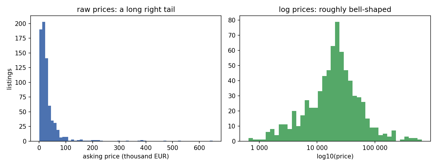
Prices are spread over three orders of magnitude. On a raw scale a handful of luxury cars dominate everything; on a log scale the distribution is a well-behaved bell. Since MAPE only cares about relative error, the log scale is the natural one: $|\log \hat y - \log y| \approx |\hat y - y|/y$ for small errors.
The title is the most informative column, but it must be parsed. "BMW 1-Series 1,6L 2014" contains the make (BMW), the model (1-Series), the engine size and the year. There are 52 makes and 217 models; some makes have two words (Land Rover, Alfa Romeo, Rolls Royce).
The data is messy, as announced. Engine size uses a decimal comma ("1,6L", or "Electric"), power is missing for 56 % of the cars, MOT is a date "11/2027" or "Not applicable" (which means the car is new), extras are a free list of up to 17 items.

A first baseline

The organisers' baseline is a random forest on year, mileage, power, seats and four label-encoded categories, trained on the raw price. In our cross-validation it scores MAPE 0.550 (20 points). It loses for two reasons: it ignores the make and model, and it minimises squared euros, so it spends its effort on the Rolls-Royces and treats a 3 000 EUR error on a 1 000 EUR car as negligible. MAPE thinks the opposite.

Fixing both, by parsing the title and predicting $\log(\text{price})$ , changes everything: a ridge regression with one-hot make and model, age, $\log$ mileage and engine size already reaches 0.275, and LightGBM on the full feature set 0.247.

The key idea

Predicting the "typical" price is not what MAPE rewards. Because MAPE punishes over-estimates more than under-estimates, the best guess is systematically below the median, and you should shrink every prediction by a constant factor.

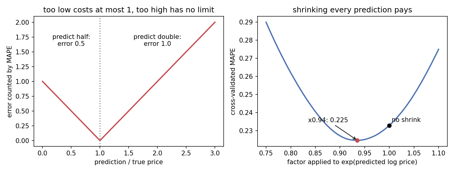
Look at the penalty for a single car (left panel below). If you predict half the true price, MAPE counts an error of 0.5. If you predict double, it counts 1.0. An under-estimate costs at most 1 (predicting 0), an over-estimate has no limit. When the model is uncertain, it is safer to lean low.

MAPE asymmetry and the effect of shrinking

We can make this exact. Suppose that, given the features, the price $Y$ is uncertain with $\log Y \sim \mathcal N(\mu, \sigma^2)$ , and we predict a constant $c$ . The expected loss is $\mathbb E\big[|Y - c| / Y\big]$ . Its derivative in $c$ is

\frac{d}{dc}\,\mathbb E\!\left[\frac{|Y-c|}{Y}\right] = \mathbb E\!\left[\frac{\operatorname{sign}(c - Y)}{Y}\right],

which vanishes when the "weight" $1/Y$ is split equally on both sides of $c$ . In other words, $c$ is the median of the distribution reweighted by $1/y$ . Multiplying the log-normal density by $1/y$ gives, after completing the square, another log-normal with mean $\mu - \sigma^2$ . Hence

c^\star = e^{\mu - \sigma^2} = \underbrace{e^{\mu}}_{\text{median}} \cdot\, e^{-\sigma^2}.

A model trained on $\log$ price estimates $\mu$ , so $e^{\hat\mu}$ is a median-type prediction and the MAPE-optimal one is $e^{-\sigma^2}$ times smaller. Our cross-validated log residuals have $\sigma \approx 0.31$ , so the theory suggests a factor $e^{-0.31^2} \approx 0.91$ . The empirical optimum (right panel) is 0.93: the residuals are more peaked and heavier-tailed than a Gaussian, but the order of magnitude is right. This single multiplication takes the MAPE from 0.234 to 0.225.

The error analysis confirms the story: the 15 worst errors are all over-estimates of very cheap cars (a 1 000 EUR car priced at 3 700, a 750 EUR car at 2 000). A car listed far below its "book value" is usually damaged or needs urgent sale, and nothing in the listing says so. Each of those costs 1.5 to 3.7 units of error, while an equally wrong under-estimate would cost less than 1.

The full solution

Parsing. Make and model from the title (with the two-word makes handled), age $= 2026 - \text{year}$ , $\log(1+\text{km})$ , km per year, engine litres (decimal comma), power, seats, doors, "MOT not applicable" flag and months until the MOT, number of extras plus flags for 8 telling ones (leather, panoramic roof, 360 camera, adaptive cruise...), city, and the raw categories.
Target encoding of make and model: the smoothed mean log price of the category, $\frac{\sum y + k\bar y}{n + k}$ with $k = 5$ pseudo-listings at the global mean, computed out of fold on the training rows so that a car never sees its own price.
Two models on $\log(\text{price})$ : LightGBM with an L1 loss (15 leaves, 600 trees, learning rate 0.03, subsampling), whose median-type behaviour suits a metric based on absolute errors; and a ridge regression on one-hot make/model/fuel/body plus standardised age, age², log mileage, engine size, MOT flag and number of extras.
Blend in log space, 0.7 LightGBM + 0.3 ridge: the two make different mistakes (the ridge extrapolates smoothly for rare models, the trees capture interactions such as "old luxury car").
Shrink: final price $= 0.93 \cdot \exp(\text{blend})$ .

pred = SHRINK * np.exp(W_LGB * fit_lgb(X, y, Xt) + (1 - W_LGB) * fit_ridge(X, y, Xt))

The shrink factor was chosen on the out-of-fold predictions. To check that this choice is not overfitted, we also chose it on 4/5 of the cars and applied it to the remaining fifth: the MAPE is the same (0.2252), and the optimum is stable at 0.93 to 0.94 for every model we tried.

Results

approach (3 x 5-fold CV on the 728 training cars)	MAPE	points
organisers' baseline: random forest on raw price	0.550	20.0
LightGBM, MAPE objective on raw price (failed)	0.303	69.4
ridge on log price, one-hot make/model	0.275	74.9
random forest on log price	0.273	75.5
LightGBM on log price, L2 loss	0.247	80.6
LightGBM on log price, L1 loss	0.242	81.7
same, model name with 2 words instead of 1 (mixed: ridge got worse)	0.237	82.6
blend 0.7 LightGBM-L1 + 0.3 ridge	0.234	83.2
blend, multiplied by 0.93 (final)	0.225	84.9

The final model reaches a cross-validated MAPE of 0.225 (84.9 points), against 0.202 for the best public leaderboard entry. The leaderboard is computed on 91 different cars; with MAPE values whose per-car standard deviation is about 0.3, a 91-car average has a standard error near 0.03, so our estimate and the top of the leaderboard are within noise of each other, but we cannot claim to match it.

A surprise: telling LightGBM to minimise MAPE directly on the raw price is clearly worse (0.303) than learning log prices. The MAPE gradient is $\pm 1/y$ , so the expensive cars get almost no weight and the boosting starts from a poor constant; the log transform gives a much better-conditioned problem, and the shrink then corrects the one thing it gets wrong.

What to remember

Match the target to the metric. For a relative-error metric, learn $\log y$ : errors on cheap and expensive items then count the same, as in the metric.
The best prediction depends on the loss, not only on the data. Squared error wants the mean, absolute error the median, MAPE a $1/y$ -weighted median that lies below both. For a log-normal uncertainty, that is the median times $e^{-\sigma^2}$ .
Post-processing is part of the model. One constant factor, checked with a nested split, was worth as much as all the feature engineering after the first parse.
Free text hides the best features. Parsing the title into make and model mattered more than any choice of algorithm.
Small test sets make leaderboards noisy. With 91 cars, differences of 0.02 in MAPE are mostly luck; trust a repeated cross-validation instead.

"""Cyprus Cars Price Oracle (Cyprus AI Camp 2026): predict used-car asking prices, scored by MAPE.

Files train.csv / test.csv from the Kaggle competition in the working folder. Test prices are
private: we report 3 x 5-fold cross-validated MAPE on the 728 training listings.

Pipeline
  1. parse the messy columns (make/model from the title, engine litres, MOT months, extras...);
  2. learn log(price): LightGBM with an L1 loss + a ridge regression on one-hot make/model;
  3. blend 0.7 / 0.3 in log space;
  4. multiply by 0.93: under MAPE the best constant guess is below the median (see correction).
Usage: python solution.py   -> prints the CV score and writes submission.csv
"""
import warnings
import numpy as np, pandas as pd
import lightgbm as lgb
from sklearn.linear_model import Ridge
from sklearn.model_selection import KFold
warnings.filterwarnings("ignore")

TWO_WORD_MAKES = ["Land Rover", "Alfa Romeo", "Rolls Royce", "Aston Martin"]
CATS = ["make", "model", "city", "Drive", "Colour", "Gearbox", "Body type", "Fuel type"]
SHRINK, W_LGB = 0.93, 0.7


def parse(df):
    f = pd.DataFrame(index=df.index)
    # "BMW 1-Series 1,6L 2014" -> make "BMW", model "BMW 1-Series"
    body = (df.title.str.replace(r"\s+\d{4}$", "", regex=True)
            .str.replace(r"\s+\d+,\d+L$", "", regex=True).str.replace(",", "", regex=False).str.strip())
    f["make"] = [next((m for m in TWO_WORD_MAKES if b.startswith(m)), b.split()[0]) for b in body]
    f["model"] = [m + " " + (b[len(m):].split() or [""])[0] for b, m in zip(body, f.make)]
    f["age"] = 2026 - df.Year
    f["logkm"] = np.log1p(df["Mileage (in km)"])
    f["km_per_year"] = df["Mileage (in km)"] / (f.age + 0.5)
    f["engine"] = pd.to_numeric(df["Engine size"].str.replace("L", "").str.replace(",", "."), errors="coerce")
    f["power"] = df.Power
    f["seats"] = df.Seats
    f["doors"] = df.Doors.astype(str).str[0].map({"2": 2, "4": 4}).astype(float)
    mot = df["MOT till"].astype(str)
    f["mot_na"] = (mot == "Not applicable").astype(int)          # new or nearly new car
    f["mot_months"] = (pd.to_numeric(mot.str[-4:], errors="coerce") - 2026) * 12 + pd.to_numeric(mot.str[:2], errors="coerce")
    ex = df.Extras.fillna("")
    f["n_extras"] = ex.map(lambda s: len([x for x in s.split(",") if x.strip()]))
    for e in ["Leather seats", "Panoramic roof", "Sunroof", "360 View Camera", "Adaptive Cruise Control",
              "Lane Assist", "Heated seats", "Keyless start"]:
        f["x_" + e] = ex.str.contains(e).astype(int)
    f["city"] = df.location.str.split(",").str[0]
    for c in ["Drive", "Colour", "Gearbox", "Body type", "Fuel type"]:
        f[c] = df[c].astype(str)
    return f


def target_encode(Xa, ya, Xb, col, k=5):
    """smoothed mean log price of each make / model (k pseudo-listings at the global mean)"""
    g = pd.DataFrame({"c": Xa[col].values, "y": ya}).groupby("c").y.agg(["sum", "count"])
    return Xb[col].map((g["sum"] + k * ya.mean()) / (g["count"] + k)).fillna(ya.mean()).values


def with_te(Xa, ya, Xb, inner_oof):
    Xb = Xb.copy()
    for col in ["make", "model"]:
        if inner_oof:      # encoding the training rows: out-of-fold, so a row never sees its own price
            v = np.zeros(len(Xa))
            for a, b in KFold(5, shuffle=True, random_state=1).split(Xa):
                v[b] = target_encode(Xa.iloc[a], ya[a], Xa.iloc[b], col)
            Xb["te_" + col] = v
        else:
            Xb["te_" + col] = target_encode(Xa, ya, Xb, col)
    return Xb


def fit_lgb(Xa, ya, Xb):
    A, B = with_te(Xa, ya, Xa, True), with_te(Xa, ya, Xb, False)
    for c in CATS:
        A[c] = A[c].astype("category")
        B[c] = pd.Categorical(B[c], categories=A[c].cat.categories)
    m = lgb.LGBMRegressor(objective="l1", n_estimators=600, learning_rate=0.03, num_leaves=15,
                          min_child_samples=5, subsample=0.8, subsample_freq=1, colsample_bytree=0.7,
                          reg_lambda=1.0, cat_smooth=10, min_data_per_group=5, verbose=-1, n_jobs=2)
    return m.fit(A, ya).predict(B)


def fit_ridge(Xa, ya, Xb):
    cols = ["age", "logkm", "engine", "mot_na", "n_extras"]
    A, B = Xa[cols].copy(), Xb[cols].copy()
    med = A.median(); A, B = A.fillna(med), B.fillna(med)
    A["age2"], B["age2"] = A.age ** 2, B.age ** 2
    mu, sd = A.mean(), A.std() + 1e-9
    A, B = (A - mu) / sd, (B - mu) / sd
    cat = ["make", "model", "Fuel type", "Body type"]
    oh = pd.get_dummies(pd.concat([Xa[cat], Xb[cat]]).astype(str)).astype(float).values
    A = np.hstack([A.values, oh[:len(Xa)]]); B = np.hstack([B.values, oh[len(Xa):]])
    return Ridge(alpha=1.0).fit(A, ya).predict(B)


def predict_log(Xa, ya, Xb):
    return W_LGB * fit_lgb(Xa, ya, Xb) + (1 - W_LGB) * fit_ridge(Xa, ya, Xb)


def mape(t, p):
    return np.mean(np.abs(t - p) / t)


if __name__ == "__main__":
    tr, te = pd.read_csv("train.csv"), pd.read_csv("test.csv")
    X, Xt, y = parse(tr), parse(te), np.log(tr.price.values)
    scores = []
    for r in range(3):
        oof = np.zeros(len(X))
        for a, b in KFold(5, shuffle=True, random_state=r).split(X):
            oof[b] = predict_log(X.iloc[a], y[a], X.iloc[b])
        scores.append((mape(tr.price.values, np.exp(oof)), mape(tr.price.values, SHRINK * np.exp(oof))))
    s = np.array(scores)
    print(f"CV MAPE: median-style {s[:, 0].mean():.4f}, shrunk x{SHRINK} {s[:, 1].mean():.4f}"
          f" -> points {max(0, min(100, (0.65 - s[:, 1].mean()) * 200)):.1f}")
    pred = SHRINK * np.exp(predict_log(X, y, Xt))
    pd.DataFrame({"Id": te.Id, "price": pred.round(0)}).to_csv("submission.csv", index=False)