Cuties Segmentation

The problem in brief

Each image shows a cat or a dog, one of 37 breeds, and you must output a binary mask: 1 on the animal, 0 elsewhere. The catch is in the rules. The only pretrained model allowed is CLIP ViT-B/16 (openai/clip-vit-base-patch16), a model trained to match whole images with captions that was never trained to segment anything, and you get just 20 images with masks. Prompts are free, and training on the 20 images is allowed. The official version had 1 000 test images, scored on Kaggle.

The Kaggle files need a login, so we rebuilt the task from its public source, the Oxford-IIIT Pet dataset (the 37 breeds and the trimap masks match the statement). We drew 20 labelled images at random from the official trainval list and 500 test images from the official test list (seed 0). The ground truth is the pet plus its outline band (trimap value "not background"). All scores below are on this rebuilt test set, not the official Kaggle one, and every choice was made using only the 20 labelled images.

How you are scored

The baseline notebook states that the score is the mean IoU of the binary masks. For one image with predicted mask $\hat{M}$ and true mask $M$:

$$\text{IoU} = \frac{\lvert \hat{M} \cap M \rvert}{\lvert \hat{M} \cup M \rvert}, \qquad \text{score} = \frac{1}{N}\sum_{i=1}^{N} \text{IoU}_i .$$

We report the mean IoU of the pet mask, and also the two-class mean IoU (average of the pet IoU and the background IoU), since the exact Kaggle convention is not public. Both lead to the same conclusions. No threshold is published and the leaderboard needs a login, so there is no official target. As a reference, the trivial "whole image is the pet" mask gives a pet IoU of 0.42 on this data.

First look at the data

The Oxford pets are friendly images for this task: one animal per image, usually large and centred. The pet covers 42 % of the picture on average, the backgrounds are sofas, grass, floors, beds. The difficulty lies elsewhere.

CLIP was trained with a contrastive loss between a global image embedding (the class token) and a caption. Nothing in that objective asks the 196 patch tokens to stay "about" their own location. So the obvious approach does not work: take the final patch tokens, project them into the text space and compare each with "a photo of a cat". The last attention layers mix information across the whole image to build the global embedding, and every final patch token ends up saying roughly "this image contains a cat". We measured it: this naive map scores a pet IoU of 0.30, worse than predicting the whole image. It is a classic surprise with CLIP: the final patch tokens are so globally mixed that their map no longer tells the animal from its surroundings.

Two things make the problem solvable:

1. Intermediate layers are still local. Earlier transformer blocks have not yet mixed everything, so a patch token from layer 8 still describes its own 16×16 patch, but already with rich semantics (fur, ear, eye).
2. The value path of the last block is local too. That is the MaskCLIP trick (Zhou et al., 2022), our zero-shot baseline.

Resolution matters. At CLIP's native 224 px, a ViT-B/16 gives a 14×14 grid of patches, too coarse for a mask. We feed 448 px images and interpolate the position embeddings (interpolate_pos_encoding=True), which gives 28×28 patches of 16 pixels.

A first baseline

Zero-shot MaskCLIP, no training at all. In the last transformer block, the attention output for each patch is a weighted mix of the value vectors of all patches. MaskCLIP drops the query-key weighting and keeps, for each patch, its own value vector, passed through the output projection, the final layer norm and CLIP's visual projection. The result lives in the joint image-text space but stays local. We compare each patch with 51 prompts: "a photo of a {breed}, a type of pet." for the 37 breeds, and "a photo of {grass, floor, sofa, wall, ...}." for 14 background words. Softmax over the 51 classes, then sum the 37 breed probabilities to get $P(\text{pet})$ per patch, upsample bilinearly to the image size, and threshold.

Result: pet IoU 0.751 on test (two-class mIoU 0.782). The figure below shows its typical look: the right region, but ragged, with holes and islands, because each patch decides alone from a single noisy embedding.

The key idea

Treat frozen CLIP as a feature extractor and learn a linear classifier per patch: 20 images are not 20 examples, they are 15 680.

Each labelled image gives $28 \times 28 = 784$ patches, each with a 768-dimensional token and a label (pet if more than half its pixels are pet). A logistic regression on these 15 680 examples is a tiny model, 769 parameters, and it is learned in seconds.

Two choices decide the score, and both were made by grouped cross-validation on the 20 images: 5 folds of 4 images, never splitting the patches of one image between training and validation. Neighbouring patches of the same image are nearly identical, so a patch-level split would leak and look far too optimistic.

features	C = 0.001	C = 0.01	C = 0.1
layer 8 tokens	0.876	0.862	0.818
layer 12 (final) tokens	0.861	0.843	0.784

(grouped-CV pet IoU on the 20 labelled images)

• Strong regularisation wins. With 768 features and examples from only 16 training images, a weakly regularised model memorises those images' colours and backgrounds. A small $C$ (strong L2 penalty) forces it to use the few directions that generalise.
• Layer 8 beats layer 12, as the "locality" argument predicts. We also tried concatenating layers 4, 8 and 12 (0.871): no gain over layer 8 alone.

Then use what you know about the shape. One image contains one animal, as a single blob without holes. So we keep the largest connected component and fill its holes. Grouped CV: 0.876 → 0.888. This is the kind of prior knowledge a model learnt from 20 images cannot discover alone.

The full solution

1. Resize each image to 448×448, normalise with CLIP's mean and standard deviation, and run the frozen vision tower with interpolated position embeddings.
2. Keep the 784 patch tokens after block 8, and the MaskCLIP pet probability from block 12 for the baseline.
3. Build patch labels for the 20 images: average-pool the true mask over each 16×16 patch, label = share > 0.5.
4. Standardise the tokens and fit LogisticRegression(C=0.001) on the 15 680 labelled patches.
5. For a test image, predict $P(\text{pet})$ for each of its 784 patches, upsample the 28×28 map bilinearly to the original resolution (soft boundaries are better than 16-pixel blocks), and threshold at 0.5.
6. Keep the largest connected component and fill holes.

h = V.pre_layrnorm(V.embeddings(x, interpolate_pos_encoding=True))   # 448 px -> 1 + 28*28 tokens
for i, layer in enumerate(V.encoder.layers):
    h = layer(h, None)
    if i + 1 == 8: tokens = h[0, 1:]                                 # drop the class token

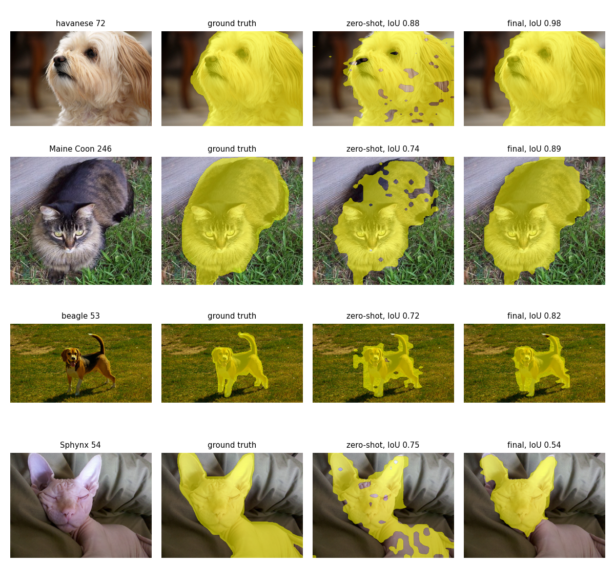
The examples tell the story. On the Havanese and the Maine Coon, the zero-shot map has holes and spills onto the background, while the final mask is clean. On the beagle, MaskCLIP's 16-pixel blocks merge the thin legs and tail with the grass, and the probe outlines them much better. The Sphynx (last row) is the instructive failure: a hairless pink cat lying on a person's arm. The probe learned from 20 images that "pet" means fur, so it keeps the head and loses the hairless body, which looks like the skin of the hand around it (IoU 0.54). The zero-shot model does better on this image (0.75), because its text prompt "a photo of a sphynx" carries knowledge of the breed that 20 images do not.

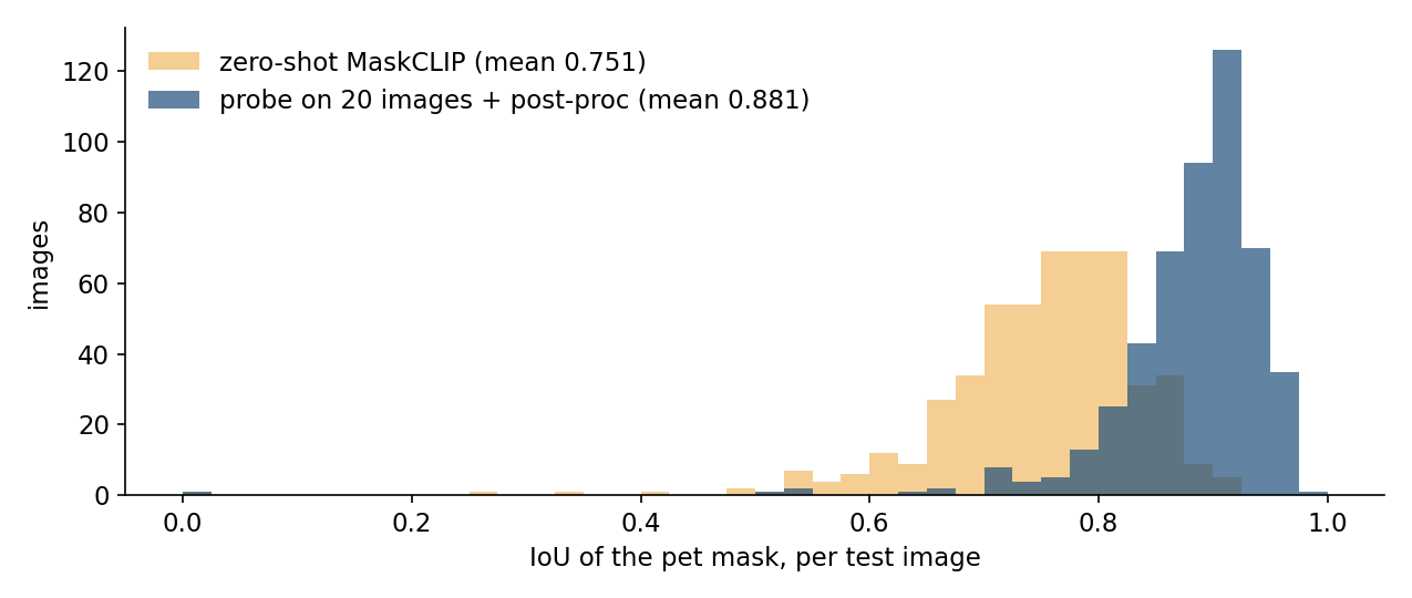
Over the 500 test images the final model's median IoU is 0.89, and only 1 image is below 0.5, against 6 for the zero-shot baseline. Cats and dogs are segmented about equally well (0.878 against 0.883).

Results

approach	grouped CV on the 20 images	test pet IoU	test 2-class mIoU
whole image = pet		0.420
naive: final patch tokens against the text prompts		0.301	0.313
zero-shot MaskCLIP, breed and background prompts		0.751	0.782
linear probe, layer 12, C = 0.001	0.861	0.873	0.886
linear probe, layers 4 + 8 + 12	0.871
linear probe, layer 8, C = 0.1 (weak regularisation)	0.818
linear probe, layer 8, C = 0.001	0.876	0.873	0.885
+ largest blob, fill holes (final)	0.888	0.881	0.894

(blank cells: not evaluated on test, to avoid choosing on it)

The final pipeline reaches a pet IoU of 0.881 on our 500 rebuilt test images, with CPU only: about 0.6 s per image for the CLIP forward pass, and a few seconds of training. On test, layers 8 and 12 end up tied (0.873): the 0.015 CV gap was partly noise from 20 images, which is a useful reminder of how little 20 images can tell apart.

Ideas we did not have time to test, natural next steps: horizontal-flip test-time augmentation; adding the MaskCLIP probability as an extra feature (a quick try gave no gain in CV); and refining boundaries with colour, for instance a CRF or a guided filter, since the 16-pixel patch grid is now the main source of error along the edges.

What to remember

• A model trained on global captions can still segment, if you read the right layer. Final CLIP patch tokens are globally mixed; intermediate tokens (layer 8) and the value path of the last block (MaskCLIP) stay local.
• Few images can mean many examples. 20 masks give 15 680 labelled patches. A linear probe on frozen features is the right size of model for that data.
• Cross-validate by group. Patches of one image are near-duplicates: split by image, or your validation score will lie.
• Regularise hard when features are many and sources few. $C = 0.001$ beat $C = 0.1$ by 6 points.
• Add the priors you know. "One animal, no holes" became a two-line post-processing step worth almost a point, and it is knowledge that 20 images could not have taught the model.