AI Fundamentals Challenge

The problem in brief

This is the first round of the 2025 Canadian AI Olympiad national qualifier: a 35-question objective test. Questions 1 to 25 are multiple choice (one correct option out of five) on NumPy and pandas behaviour, the calculus of linear regression, optimisation, the bias-variance trade-off, classical models (trees, SVMs, naive Bayes, K-means) and graph search. Questions 26 to 35 are short "fill in the blank" or "compute this number" items: small pandas pipelines, a cost function, an information gain, a naive Bayes posterior, two gradient loops and a crawling question. Nothing here is hard on its own; the difficulty is to be fast and exact on 35 different topics.

How you are scored

Each multiple-choice question is worth 2 points and each open question 5 points, for a total of

$$25 \times 2 + 10 \times 5 = 100 \text{ points.}$$

Numeric answers are typed into a box with a character limit (for example 3 to 4 characters for "two decimal places"), so the rounding format matters. No official answer key was published with the paper; every answer below is derived from scratch, and every computable one is checked independently in solution.py (finite differences for gradients, exact fractions for probabilities, running the code for the pandas questions).

Question by question

Part A: code and arrays (Q1, Q2, Q7, Q14, Q25)

Q1. np.dot(A, B.T) multiplies each row of $A$ by each row of $B$ (the columns of $B^\top$ are the rows of $B$), so $C_{ij} = a_i \cdot b_j$:

$$C_{00} = 1\cdot1+2\cdot0+3\cdot5 = 16,\quad C_{01} = 2+2+18 = 22,\quad C_{10} = 0+0+20 = 20,\quad C_{11} = 0+1+24 = 25 .$$

C[:2, :2] is the top-left block: [[16 22] [20 25]]. The trap option [[16 20] [22 25]] is its transpose, the block of B @ A.T: what you get by mixing up which matrix provides the rows.

Q2. df['B'] > 20 keeps rows 2, 3, 4; the column list keeps A and C. iloc[1, 1] is the second kept row (original row 3) and the second kept column (C), whose value is 2. loc filters by labels, iloc then counts positions in the filtered result.

Q7. i takes the values $1, 3, 9, \dots, 3^k$ and the loop stops once $3^k > n$, so it runs $\lfloor \log_3 n \rfloor + 1$ times: $O(\log_3 N)$. (Mathematically $O(\log_3 N) = O(\log_2 N)$ since the bases differ by a constant factor, but the option matching the code is $\log_3$.)

Q14. fillna(0) returns a new series used only to build C; column B itself still contains NaN. Row 1 is therefore A = 2.0, B = NaN, C = 2 + 0 = 2.0 (all floats because the column with NaN is float64): A 2.0, B NaN, C 2.0.

Q25. Vectorised NumPy runs the loop in compiled code over whole arrays (with SIMD instructions and no Python interpreter overhead per element): vectorization allows parallel operations on entire data. It does not change the maths, the learning rate or the data, and NumPy does not move anything to a GPU.

Part B: linear regression and gradient descent (Q3, Q4, Q5, Q6, Q15, Q28, Q33, Q34)

Q3. Differentiate each squared residual with the chain rule. With $r_i = y_i - (w x_i + b)$, $\partial r_i / \partial w = -x_i$, so

$$\frac{\partial L}{\partial w} = \frac{1}{n}\sum_i 2 r_i \cdot(-x_i) = -\frac{2}{n}\sum_i x_i\big(y_i - (w x_i + b)\big).$$

Two traps: forgetting the factor $x_i$ (that is $\partial L/\partial b$) and forgetting the minus sign.

Q4. $(X^\top X)^{-1}$ must exist: $X^\top X$ is invertible, which means the columns of $X$ are linearly independent (no duplicated or perfectly collinear feature, and at least as many samples as features). $y$ can be anything and $X$ is usually not even square, so "symmetric" or "orthogonal" make no sense here.

Q5. In matrix form $L(w) = \frac{1}{n}\lVert Xw - y\rVert^2$, whose gradient is $\frac{2}{n}X^\top(Xw - y)$. Gradient descent moves against it: $w := w - \frac{2\alpha}{n}X^\top(Xw-y)$. A quick shape check eliminates the others: with $X$ of shape $(n, d)$, $X^\top(Xw-y)$ has shape $(d,)$ like $w$, while $(Xw-y)X^\top$ does not even multiply.

Q6. When one feature is in thousands and another in fractions, the loss surface is a long thin valley: one learning rate is too big along one axis and too small along the other. Standardising puts features on the same scale and centres them at 0, which avoids huge gradient steps in one direction. It does not decorrelate features (that would be PCA whitening) and trees do not care about scaling.

Q15. With too large a step, each update overshoots the minimum, landing higher on the other side: the cost oscillates or diverges.

Q28. With $f(x) = 6x + 4$ the predictions are $10, 16, 22, 28, 34$ and the errors $f(x) - y$ are $0, -1, -3, -4, -1$:

$$J = \frac{1}{2\cdot 5}(0 + 1 + 9 + 16 + 1) = \frac{27}{10} = \boxed{2.7}.$$

Q33. Inside the loop:

f_wb = w * x[i] + b
cost = (f_wb - y[i]) ** 2
cost_sum = cost_sum + cost

On the Q28 data this function returns exactly 2.7, a nice cross-check.

Q34. Same structure, but the prediction goes through the sigmoid and the gradient accumulates the error times each feature:

for i in range(m):
    f_wb_i = 1 / (1 + np.exp(-(np.dot(X[i], w) + b)))
    err_i = f_wb_i - y[i]
    for j in range(n):
        dj_dw[j] = dj_dw[j] + err_i * X[i, j]
    dj_db = dj_db + err_i
dj_dw = dj_dw / m
dj_db = dj_db / m

The remarkable fact this question hides: for logistic regression with cross-entropy, the gradient has exactly the same form as for linear regression with MSE, $\frac{1}{m}\sum_i (f(x^{(i)}) - y^{(i)})x^{(i)}_j$; only $f$ changes. solution.py checks the loop against the vectorised formula $\frac{1}{m}X^\top(\sigma(Xw+b) - y)$.

Part C: generalisation (Q9, Q10, Q16, Q17, Q18, Q21, Q22, Q24)

These eight questions are one idea seen from several angles. The test error of a model splits (for squared loss) into

$$\mathbb{E}\big[(y - \hat f(x))^2\big] = \text{bias}^2 + \text{variance} + \text{noise}.$$

A rigid model has high bias (wrong on average, even on training data); a very flexible one has high variance (it changes a lot when the training set changes, so it fits noise).

question	situation	answer
Q9	huge regularisation $\lambda$	weights forced near 0: underfit
Q16	the trade-off in one sentence	reducing bias often increases variance ("always" in another option is too strong)
Q17	train and validation errors meet at a high value	more data will not help: underfitting
Q18	adding $\frac{\lambda}{2}\lVert w\rVert^2$	shrinks weights: increases bias, decreases variance (L2 never sets weights exactly to 0, L1 does)
Q21	deep tree, few samples per leaf	each leaf memorises a handful of points: overfitting
Q22	high variance looks like	low training error, high test error
Q24	$J_{cv} \gg J_{train}$	high variance
Q10	smaller XGBoost learning rate $\eta$	each tree corrects less, so you need more trees but generalise better (shrinkage is a regulariser)

Part D: classical models (Q8, Q13, Q19, Q20, Q23, Q30, Q31)

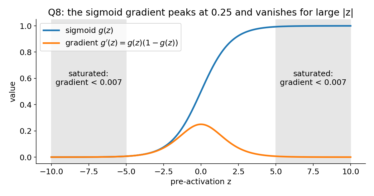
Q8. $g'(z) = g(z)(1 - g(z))$ is at most $0.25$ (at $z=0$) and decays like $e^{-|z|}$: the gradient approaches zero (vanishes). This is why deep sigmoid networks trained slowly, and why ReLU became standard.

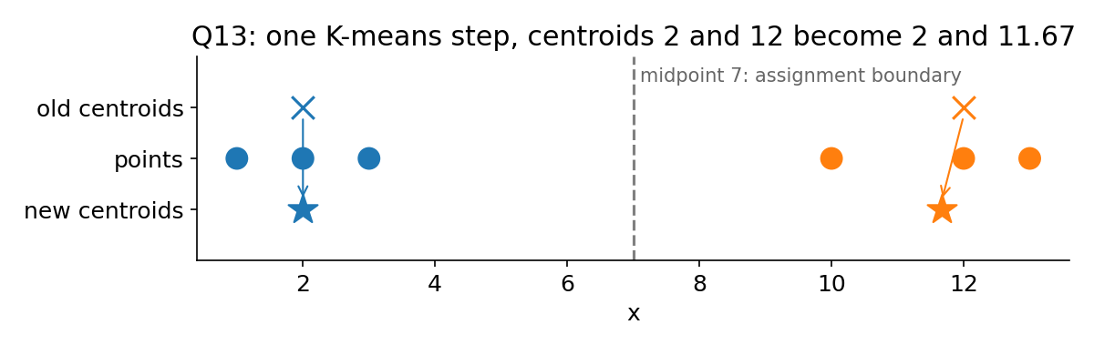
Q13. Assignment: the boundary between centroids 2 and 12 is their midpoint 7, so $\{1,2,3\}$ go to $C_1$ and $\{10,12,13\}$ to $C_2$. Update: $C_1 = 6/3 = 2$ and $C_2 = 35/3 \approx 11.67$: $C_1 = 2$, $C_2 = 11.67$ (the option printed with a stray "A." prefix).

Q19. We want the statement that is false as a limitation. SVMs maximise the margin, which controls capacity independently of the dimension; that is exactly why linear SVMs work so well on text, where features vastly outnumber samples. So "SVMs suffer from severe overfitting when the feature dimension is higher than the number of samples" is not a real limitation. The other four are (scaling sensitivity, tuning of $C$ and kernel parameters, no native probabilities, training cost growing at least quadratically with $n$).

Q20. A kernel $k(x, x') = \varphi(x)\cdot\varphi(x')$ gives dot products in feature space without computing the mapping $\varphi$. The boundary is linear in feature space but nonlinear in input space (the reverse of one distractor), and the trick lives inside the dual formulation.

Q23. Naive Bayes is a generative model: it estimates the likelihood $P(x_i \mid C_k)$ of each feature given the class, then flips it with Bayes' rule. Logistic regression is discriminative: what it estimates is $P(C_k \mid x)$, never how the features are distributed. Plugging such a number where Bayes' rule expects $P(x_i \mid C_k)$ means the factors are no longer likelihoods, so you lose likelihood estimation (the generative view of the data). This question is the least clear-cut of the paper; "conditional independence" is the tempting distractor, but that assumption is about how the factors are combined (by a product), which you keep.

Q30. Entropy in bits, $H(p) = -\sum_c p_c \log_2 p_c$:

$$H(\text{parent}) = H(0.6, 0.4) = 0.6(0.737) + 0.4(1.322) = 0.971$$ $$H(\text{left}) = H(0.8, 0.2) = 0.8(0.322) + 0.2(2.322) = 0.722,\qquad H(\text{right}) = H(0.4, 0.6) = 0.971 .$$

Both branches hold 5 of the 10 samples, so

$$IG = 0.971 - \left(\tfrac{5}{10}\,0.722 + \tfrac{5}{10}\,0.971\right) = 0.971 - 0.846 = 0.1245 \approx \boxed{0.12}.$$

Careful with rounding: rounding the intermediate entropies to 0.97, 0.72, 0.97 first gives $0.125$, which then rounds to 0.13. Keep three decimals until the end.

Q31. With Laplace smoothing $\alpha=1$ and a vocabulary of $V = 3$ words, $P(w \mid c) = \frac{\text{count}(w, c) + 1}{N_c + 3}$, so the denominators are 18:

$$P(E)\,P(\text{economy}\mid E)\,P(\text{goal}\mid E) = 0.5 \cdot \tfrac{9}{18}\cdot\tfrac{5}{18},\qquad P(S)\,P(\text{economy}\mid S)\,P(\text{goal}\mid S) = 0.5 \cdot \tfrac{3}{18}\cdot\tfrac{7}{18}.$$

Normalising, the common factors cancel:

$$P(E \mid \text{doc}) = \frac{9\cdot 5}{9\cdot5 + 3\cdot 7} = \frac{45}{66} = \frac{15}{22} \approx \boxed{0.68}.$$

Part E: search (Q11, Q12, Q35)

Q11. With $w > 1$ the heuristic is inflated, so the search is greedier: it expands far fewer nodes, but an inflated heuristic is no longer admissible. Faster but possibly sub-optimal (the cost found is at most $w$ times the optimum when $h$ is admissible).

Q12. Uniform Cost Search (Dijkstra) stops as soon as the goal is popped from the priority queue, which is correct only if path costs can never decrease later. A negative edge breaks that: a cheaper path through a not-yet-expanded node may still exist. So it terminates early with an incorrect cost. (An infinite loop needs a negative cycle and no visited set: possible, but not what happens in general.)

Q35. BFS with a visited set. All links have the same "cost", and we want every page, not a cheapest path, so UCS and A* bring nothing (no edge weights, no goal, no heuristic). BFS explores the site level by level from the home page, which reaches the important, shallow pages first and is easy to cap at a depth; the visited set is essential because the web graph has cycles (every page links back to the home page). DFS with a visited set would also visit everything, but it dives into deep chains of links (calendars, pagination) and needs care with recursion depth, so BFS is the safer default.

Part F: pandas and scikit-learn fill-ins (Q26, Q27, Q29, Q32)

Q26.

df = pd.read_csv('temperature.csv')
df['temp_f'] = np.array(df['temp_c']) * 9 / 5 + 32
plt.plot(df['day'], df['temp_f'], marker='o')
plt.xlabel('Day'); plt.ylabel('Temperature (°F)'); plt.title('Daily temperature')
plt.show()

(Values: 53.6, 57.2, 59.0, 51.8, 55.4 °F.)

Q27. In order: fillna(0), mean(), fillna(mean_discount), df['units_sold'] * df['price'] * (1 - df['discount']), groupby, sort_values. Order matters: the mean discount is computed before filling (pandas skips NaN in mean), otherwise you would average the filled values.

Q29.

nan_counts = df.isna().sum()
cols_sorted = nan_counts.sort_values(ascending=False).index.tolist()
pct = df.isna().mean().mul(100).sort_values(ascending=False)
pct = pct[pct >= 20]
plt.bar(pct.index, pct.values); plt.xticks(rotation=90)
plt.xlabel('column'); plt.ylabel('% NaN'); plt.show()

isna().mean() is the fraction of missing values per column, because True counts as 1.

Q32. In order: LogisticRegression, accuracy_score, LogisticRegression, fit, predict, accuracy_score.

The key idea

The paper looks like 35 unrelated facts, but most of it rests on three reflexes:

1. Derive, do not recall. Q3, Q5, Q28, Q30, Q31, Q33 and Q34 are a single chain rule or a single formula applied carefully. Writing the residual $r_i$ and its derivative takes ten seconds and removes every sign trap; a shape check ($X^\top$ of shape $(d, n)$ times a vector of shape $(n,)$) eliminates impossible options in Q5 instantly.
2. One picture for generalisation. Training error measures bias, the gap between validation and training error measures variance. Q9, Q10, Q16, Q17, Q18, Q21, Q22 and Q24 are all read off that picture.
3. Know what each method assumes. UCS assumes non-negative costs (Q12), A* optimality assumes an admissible heuristic (Q11), the normal equation assumes independent columns (Q4), naive Bayes estimates likelihoods (Q23). A question asking "what happens if..." is almost always "which assumption breaks".

The full solution

solution.py contains an assert for every computable answer: the matrix block of Q1, the pandas outputs of Q2, Q14, Q26, Q27, Q29, finite-difference checks of the gradients of Q3 and Q5, an iteration counter for Q7, the K-means step of Q13, exact fractions for Q28 and Q31, the entropy computation of Q30, a small logistic regression pipeline for Q32 and the loop implementations of Q33 and Q34 compared with their vectorised versions. It also draws the two figures.

Results

Q	answer	Q	answer
1	[[16 22] [20 25]]	19	overfitting when $d > n$ (not a real limitation)
2	2	20	dot products in feature space without the mapping
3	$-\frac{2}{n}\sum_i x_i(y_i-(wx_i+b))$	21	deep tree with few samples per leaf
4	$X^\top X$ invertible	22	low training error, high test error
5	$w := w - \frac{2\alpha}{n}X^\top(Xw-y)$	23	likelihood estimation (least certain)
6	centres features, avoids large gradient steps	24	high variance
7	$O(\log_3 N)$	25	parallel operations on entire data
8	approaches zero (vanishes)	26	read_csv, * 9 / 5 + 32, plot
9	underfit	27	fillna(0), mean(), fillna(...), product, groupby, sort_values
10	more trees, better generalisation	28	2.7
11	faster, possibly sub-optimal	29	isna().sum(), sort, isna().mean()*100 >= 20, bar plot
12	terminates early with incorrect cost	30	0.12
13	$C_1 = 2$, $C_2 = 11.67$	31	0.68
14	A 2.0, B NaN, C 2.0	32	LogisticRegression, accuracy_score, fit, predict
15	oscillates or diverges	33	f_wb, squared error, accumulate
16	reducing bias often increases variance	34	sigmoid prediction, error, accumulate, divide by $m$
17	underfitting	35	BFS with a visited set
18	increases bias, decreases variance

Typical mistakes worth naming: the transposed matrix in Q1 (forgetting .T), thinking fillna modifies the column in place in Q14, rounding intermediate entropies in Q30 (gives 0.13), and forgetting that Laplace smoothing adds the vocabulary size to the denominator in Q31.

What to remember

• Check shapes and signs before picking an option. Most wrong options in gradient questions fail a shape check or a sign check.
• Training error tells you about bias, the train/validation gap tells you about variance. Regularisation, shallower trees and smaller learning rates trade the second for the first.
• Keep full precision until the last step, then round in the format requested: a two-decimal answer box punishes early rounding.
• pandas returns new objects (fillna, sort_values) unless you assign them back; loc is by label, iloc by position in the current result.
• Every algorithm comes with an assumption (non-negative costs, admissible heuristic, invertible $X^\top X$): "what happens if" questions are about which one breaks.